Author Archives: dev

Animal Models of Tinnitus: A Review

Synopsis

Animal models have significantly contributed to understanding the pathophysiology of chronic subjective tinnitus. They are useful because they control etiology, which in humans is heterogeneous; employ random group assignment; and often use methods not permissible in human studies. Animal models can be broadly categorized as either operant, or reflexive, based on methodology. Operant methods use variants of established psychophysical procedures to reveal what an animal hears. Reflexive methods do the same using elicited behavior, e.g., the acoustic startle reflex. All methods contrast the absence of sound and presence of sound, since tinnitus cannot by definition be perceived as silence.

Keywords

Animal models, acoustic startle reflex, operant behavioral methods, tinnitus, psychophysics

Key Points

At present there is no standard animal model of tinnitus. Two contemporary types of models are reflexive and operant; each has positive and negative features.
Reflexive models trace their origin to an experiment of Turner et al. [1]; operant models trace theirs to an experiment of Jastreboff et al. [2].
Caution is advised to distinguish between animal tinnitus studies that independently confirm the presence of tinnitus, and those that do not.

Introduction

Tinnitus in the present review refers to chronic subjective tinnitus, which has no identifiable acoustic correlate. Despite the common name, “ringing in the ears,” its source(s) appear to be primarily in the central nervous system rather than the auditory periphery. Acute tinnitus commonly follows a single exposure to high-level sound or a high dose of aspirin, and typically resolves within minutes to hours. As such it is not of medical concern. In contrast, chronic tinnitus, estimated to affect 35 – 50 million adults in the US [3], most commonly follows auditory trauma or chronic hearing loss and often persists for a lifetime[4]. It has been estimated that about five percent of those experiencing chronic tinnitus seek medical treatment. Although common, and recognized since the time of Galen [5], the pathophysiology of tinnitus is incompletely understood. This contributes to the absence of generally effective treatments, although a standard of care has been established [6, 7]. Tinnitus is typically perceived as a simple sound, a ringing or buzzing sensation, but its pathophysiology is far from simple.

Animal Tinnitus Models

Tinnitus appears to be a primitive hearing disorder. This is not to say that its pathology is simple, but rather that it derives from basic neurophysiological mechanisms likely to be present in animals as well as humans [8]. Animal models have been available since 1988 [2], and have contributed significantly to understanding the neuroscience of tinnitus[9,10]. Although animal models only approximate the human condition, their advantages over clinical studies are several. Most notably: (a) they directly control etiology, (b) they permit application of many experimental tools, from behavioral to molecular, and (c)random assignment to experimental groups enables the use of more powerful inferential statistics as well as attribution of cause. The key problem in developing an animal tinnitus model is objective and reliable assessment, rather than induction. In humans tinnitus can be induced by many conditions. These conditions have in common the reduction of peripheral signal to the brain[11–13].In animals, tinnitus has been induced using systemic treatment with salicylates [2, 14–17], ototoxic exposure [18–20], surgical disruption of the cochlea [21], and acoustic over exposure[19, 22–24]. These methods draw upon factors known to affect tinnitus in humans. The key to solving the assessment problem was provided by Jastreboff and colleagues [25]. Although tinnitus might sound like anything to an animal (or human), it can never sound like silence. All animal models of tinnitus use behavioral methods that differentiate how animals respond to sound versus silence. Typically animal studies also include one or more normal-hearing control groups. Although considerable effort has been invested in finding valid and reliable direct measures of tinnitus that do not involve behavior, at present behavioral methods are used exclusively for at least two reasons: There is no procedure for either reliably producing or determining tinnitus alone, without potential confounds. A presumptive tinnitus state might be derived from associated phenomena such as hearing loss, hyperacusis, or drug side effects. Behavioral methods enable such confounds to be more clearly sorted out. It should be noted that many presumptive tinnitus animal experiments have examined the effects of conditions likely to cause tinnitus, such as high-level sound exposure or ototoxic damage, without directly confirming the presence of tinnitus. These experiments can be informative about the consequences of auditory insults, but should be interpreted cautiously with respect to tinnitus. Not all humans exposed to acoustic trauma, or other insults develop tinnitus [26]. Similarly it has been shown that not all animals exposed to tinnitus-inducing procedures display evidence of tinnitus[27–29]. Therefore, experiments that only examine the consequence of manipulations that typically produce tinnitus, without objective confirmation, are likely to include animals without tinnitus and therefore could be reporting the effects of something other than tinnitus. Unfortunately there is no generally accepted, or standard, animal model of tinnitus against which others can be validated. Existent models have their respective strengths and weaknesses. For overview purposes, animal models can be divided into two broad categories: Models that interrogate animals about their auditory experience, and models that examine alteration of an auditory reflex. Interrogative models, hereafter called operant models, loosely following the terminology of Skinner [30], examine the effect of tinnitus on voluntary, or emitted behavior that is modified by training in an acoustic environment. These models have the general advantage of relying on auditory perception. As such, animals evaluate what they are hearing and differentially respond on the basis of their evaluation. Because operant methods require animals to report what they are hearing, they have conceptual features in common with the interrogation of humans with tinnitus, i.e., analogous to asking “what do you hear?” Operant models tap into functions in many brain areas, including areas outside those commonly defined as auditory. Although this aspect of operant models might be considered a shortcoming, it is also a strength, in that contemporary research has shown tinnitus to be mediated by widely distributed alterations in brain function[11, 31–34]. A shortcoming of operant models is that they require training and motivating subjects, interventions that can be both time consuming and requiring careful experimental control. In contrast, reflexive animal models rely on unconditioned reflexes, such as the acoustic startle response, and do not require either training or motivation management. Reflexive methods, such as sound gap inhibition of acoustic startle (GPIAS), are also rapid, and therefore well suited to determining the time course of tinnitus development. These features probably account for the current widespread use of GPIAS in animal tinnitus experiments. Although widely used, GPIAS models are not without their own issues and complexities. A further consideration is that the acoustic startle reflex, on which GPIAS is based, depends primarily on brainstem circuits [35]. Therefore the neurophysiological substrate driving the reflexive behavior assessed by GPIAS, might not have the same substrate indicated by operant models.

GPIAS Models

Animal research: More than ten years ago a new method for tinnitus screening in laboratory animals was introduced by Turner and colleagues [1]. This paradigm utilizes the acoustic startle reflex which is ubiquitously expressed in mammals and consists of contraction of the major muscles of the body following a loud and unexpected sound [36] (Fig.1, A). This reflex is reduced when preceded by a silent gap embedded in a soft background noise or tone (Fig.1, B). Gap detection is typically assessed by the ratio between the magnitude of the startle stimulus presented alone (no-gap trial) and trials in which a gap preceded startle stimulus (gap trials), also known as gap-prepulse inhibition of the acoustical startle (GPIAS) [1]. Reduced inhibition, following acoustic trauma or sodium salicylate treatments is assumed to reflect tinnitus perception: When tinnitus is qualitatively similar to the background noise, it “fills in” the gap and hence, reduces inhibition (Figure 1).

OHT-19-101_Alexander Galazyuk_F1

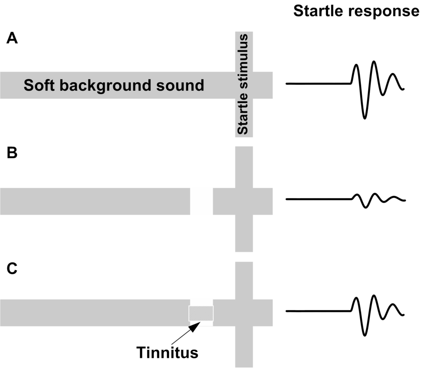
Figure 1. Schematic description of the GPIAS assay for tinnitus. A.A startle wideband noise stimulus 20 ms duration (vertical bar) is inserted into a narrowband noise or pure tone background without gap (no gap; top row) and with a gap (middle and lower rows)20 to 50 ms duration and presented 50 ms before the startle. B.An animal startle responses to the startle stimulus. The response amplitude shown by the height of the startle response waveform (top row). In animals without tinnitus, the gap greatly suppresses the startle response amplitude (middle row). In animals with tinnitus (bottom row), the gap is filled by the tinnitus (shaded rectangular within the gap) and the startle response ismuch less compared to the tinnitus free animals (middle row).

This method was enthusiastically adopted and is now widely used by many scientists in the field due to its relative simplicity over the other methods of tinnitus assessment. Since it is based on a reflex, the method is much cheaper and faster than other methods requiring training animals for weeks or months [22, 59]. It also allows for tinnitus screening of a large number of animals testing simultaneously in multiple testing boxes. Comparing of animals’ gap detection performances before and after tinnitus induction allows to separate tinnitus positive from tinnitus negative animals. The possibility of using this method for scientists with little experience in animal behavior and an opportunity to apply this methodology for tinnitus assessment in humans, made GPIAS to dominate in the field of tinnitus research. The GPIAS methodology has been improved upon over the last decade [37, 38]. It has been shown that careful considerations of GPIAS parameters such as the startle stimulus and background intensities, acoustical parameters of the gap of silence preceding the startle, and overall duration of a testing session, greatly improve results of GPIAS testing in laboratory animals [39].Recent research also demonstrated large variability in GPIAS measurements between different days of testing especially in mice [40]. Therefore averaging these results across multiple testing sessions greatly increases statistical power of the obtained data and improves the reliability of tinnitus assessments. Recent improvements to startle response magnitude assessments [41, 42] and various methods of startle response separation from animals’ ambient movements [41, 43] greatly improve GPIAS data analysis. In small rodents the whole body startle reflex is relatively easy to measure, but in larger, less active mammals, such as the guinea pig, it habituates very rapidly. Therefore the pinna reflex measurement technique has been suggested to be used instead of whole body startle reflex during GPIAS sessions [44, 45]. Despite years of using GPIAS for tinnitus assessment in various laboratory animals, the field continues to debate the original “filling-in” interpretation of the paradigm. In a study conducted on mice, the placement of the gap of silence either closer or further away from the proceeding startle stimulus could dramatically alter gap detection performance in mice [46]. Therefore the authors raised a doubt as to whether tinnitus is “filling-in” the gap, otherwise the gap placement before the startle should not have a large effect on animal’s gap detection performance. Importantly however, the most significant debates concerning GPIAS methodology on animals largely depend on successful demonstration that the method is capable of assessing tinnitus in humans.

Human research: One of the main advantages of GPIAS over other methods is that it can be used in both laboratory animals and humans [37]. Several research labs have attempted to apply GPIAS method on humans for tinnitus assessment. Eye blink was proposed to be used instead of whole body startle reflex in these studies. These experiments had a significant advantage over the animals’ studies because in humans, exact tinnitus parameters such as intensity and spectrum we can identified by tinnitus self-reports. If so, during GPIAS testing it is possible to match the background sound parameters to a person’s tinnitus characteristics which would theoretically optimize the success of the GPIAS. Unfortunately, in one of these studies it was found that gap detection performance in tinnitus patients did not depend on whether the individuals have tinnitus or not [47]. Another study showed a difference in dap detection performance between tinnitus patients and controls [48]. However this deficit was not linked to the tinnitus frequency. While these studies raised concerns and emphasized caution, they did not rule out a possibility that GPIAS deficits can indeed be interpreted as an indication of tinnitus. Indeed, if animals or humans constantly experience a phantom sound, it must still be present during the silent gap during GPIAS testing. Therefore a gap, even partially filled by tinnitus, would still be making gap detection more challenging especially when the background spectrum would closely match the spectrum of tinnitus. Further research on the improvements of GPIAS testing paradigm might help to detect gap detection challenges in tinnitus patients. The most recent work has attempted to directly measure human neurophysiological correlates of gap detection with cortical auditory evoked potentials (CAEP) recorded in the electroencephalogram (EEG) [49]. The N1 potentials in response to gaps of silence were recorded from scalp in normal tinnitus-free individuals. Such an approach does not require overt responses from the participant nor measures responses modulated by gaps. Gap-evoked cortical responses were identified in all conditions for the vast majority of participants. The N1 responses were independent on background noise frequencies or background levels. The authors recommend that this experimental design could be used in both animals and humans to identify tinnitus objectively.

Early Operant Models

A variety of operant methods for tinnitus determination in animals have been developed. Two early operant models, those developed by Jastreboff et al. [2] and Bauer et al. [22],illustrate many features common to these models. Operant models examine the effect of tinnitus on emitted behavior that has been modified by auditory training. Both methods are interrogative, in that they require subjects to respond differentially to auditory events. In the Jastreboff model, tinnitus was induced by high systemic doses of sodium salicylate. Rats were conditioned to stop licking a water spout by imposing a mild electric shock, at the end of random periods when the background sound (broad-band noise; BBN, 60 dB, SPL) was turned off, i.e., external silence. The animals were then tested with randomly-inserted silent periods, without shocks, following acute salicylate exposure (300 mg/kg). The salicylate-treated animals showed more persistent licking during the sound-off periods than controls without salicylate [2]. The interpretation was that salicylate induced tinnitus, as it is well known to do in humans, and masked the sound-off silence; therefore the rats continued to lick as they would have if sound were present. In an informative variant procedure, Jastreboff et al. demonstrated the obverse effect with animals that were lick-suppression trained while on salicylate [2]. In this variant, the rats suppressed licking more during sound-off test periods than non-salicylate controls. The interpretation was that suppression training, with tinnitus present, conditioned the animals to not lick when their tinnitus, a salient internal sound, was heard. A limitation of the Jastreboff salicylate lick-suppression model is that it was only suitable for determining acute tinnitus. Reasons for this limitation are twofold: tinnitus induced by salicylate treatment is temporary, subsiding within a day or so after discontinuing the drug, and more importantly, the tinnitus influence on licking was measured during extinction of conditioned suppression (there were no shocks when tinnitus testing).Extinction is a transient behavioral state.

A derivative operant method, well suited to assessing chronic tinnitus and still in use, was developed by Bauer and colleagues[14 22 23]. In the Bauer model, chronic tinnitus was induced using a single unilateral exposure to moderate-level tones (4 kHz at 80 dB SPL) in chinchillas, or high-level band-limited noise centered at 16 kHz (116 – 120 dB, SPL) in rats, for one hour, three or more months prior to tinnitus assessment. Unilateral exposure was used to preserve normal hearing in one ear. It also reflects a condition commonly associated with tinnitus in humans. Asymmetric acoustic trauma or hearing loss in humans is commonly associated with chronic tinnitus, including bilateral tinnitus [50]. All animals were trained to lever press for food pellets in the presence of broadband noise (BBN) (60 dB, SPL) and were tested for tinnitus using randomly introduced 1-min periods of either sound off, or tones at various levels. Lever pressing during sound-off periods was suppressed by delivering a lever-press-contingent foot shock at the end of sound-off periods. In other words, the animals could avoid the foot shock by not lever pressing during sound off. Tinnitus was indicated by decreased lever pressing when tested with tones in the vicinity of 20 kHz (Fig 2A), although tones of various frequency at various levels were tested. Control animals were not exposed to tinnitus induction but were otherwise treated and tested in parallel. The interpretation was that animals with chronic tinnitus could not hear true silence, but instead heard their tinnitus. Because they were trained to suppress lever pressing when their tinnitus was audible (during sound off periods), they suppressed lever pressing to stimulus-driven sensations that resembled their tinnitus[8, 22].Note that in the Bauer model testing and training are integrated into every session. This meant that chronic tinnitus could be measured with undiminished sensitivity over long periods. The model has been used to assess tinnitus in rats for as long as 17 months [22]. It was also found that a proportion of the exposed animals, typically 30 to 40 percent, did not develop tinnitus, although the audiometric profile of all exposed animals was equivalent (Fig. 2B).The Bauer model has also been used to determine acute tinnitus induced by systemic salicylate [14] as well as chronic tinnitus induced by ototoxic exposure [19]. (Figure 2)

OHT-19-101_Alexander Galazyuk_F2

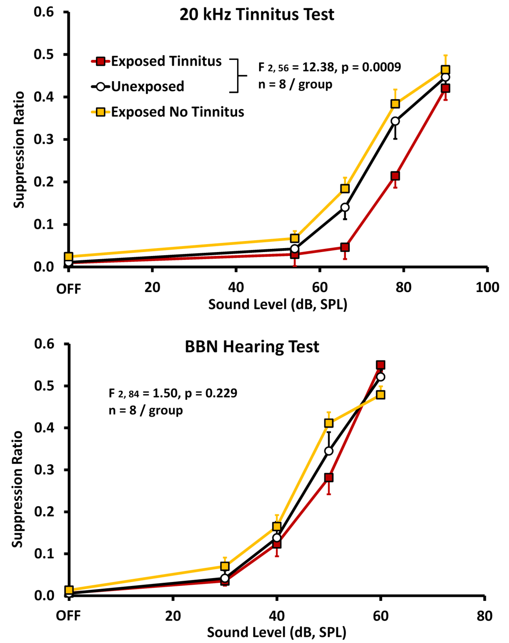
Figure 2. Psychophysical discrimination functions obtained from three groups of rats; relative lever pressing, recorded as a suppression ratio (y-axis) is plotted against test-stimulus sound level (x-axis). A suppression ratio of 0 reflects no lever presses, while a suppression ratio of 0.5 reflects lever pressing at baseline rate preceding the test stimulus. Both experimental groups (n = 8 each; filled square data points) were unilaterally exposed to band-limited noise (120 dB, SPL, octave band centered at 16 kHz) six months prior to testing. The unexposed controls (n = 8; unfilled circular data points) were trained and tested in parallel. Panel A shows the average of 5 sessions using 20 kHz test tones. A subset of exposed subjects suppressed significantly more to the 20 kHz stimuli. The statistical difference between the Exposed-with-tinnitus and Unexposed groups is shown in the inset. Suppression behavior (average of 5 sessions) of the same animals tested with broad band noise (BBN), diagnostic for free-field hearing but not tinnitus, is shown in panel B. Data points are group means averaged over 5 test sessions; error bars indicate the standard error of the mean. Significance levels were determined using a mixed analysis of variance (n = 8 per group). SPL, sound pressure level.

Operant Model Variations

Experimenters have examined a number of variations in an attempt to improve operant models. Several excellent reviews of tinnitus models may be consulted for variant features [51–53]. The extended training required by the Bauer model negatively impacts throughput, and can be shortened by employing an unconditioned indicator such as licking a spout for water. A number of researchers have adopted this modification. Zheng and colleagues developed a model that incorporated many features of the Bauer model, using water deprived rats required to lick a spout for water instead of pressing a lever for food [54]. This considerably decreased training time, although it did not decrease the time required for tinnitus to appear after acoustic induction. A wrinkle that must be addressed when substituting licking for lever pressing is the episodic nature of licking. Spontaneous pauses in licking must be taken into account, so as notto count themas false positive suppressions. Zheng et al., used shortened test sessions to reduce this error. In another operant variation, using licking behavior, May and colleagues trained rats to lick to sound resembling their tinnitus, rather than suppressing to tinnitus-like sound [55]. Chronic tinnitus was induced using high-level sound exposure while acute tinnitus was induced using high-dose salicylate treatment. Episodic features of licking were controlled by using test periods of only a few minutes, and by using a tinnitus score normalized to each animal’s non-test lick rate. They found acoustic-induced chronic tinnitus with characteristics similar to 16 kHz tones, while acute salicylate induced tinnitus was similar to narrow-band noise between 8 and 22 kHz. Licking in combination with conditioned place preference has been used to indicate chronic acoustic-induced tinnitus in hamsters [56]. Two spouts were available from which to drink, each in a distinct location; animals were trained to use the non-preferred spout in the presence of an ipsi lateral external sound. Testing occurred in silence. Licking at the sound-conditioned (non-preferred) spout indicated tinnitus [29]. Using a variant of this method, Heffner trained rats to lick from visual-and-auditory cued left or right water spouts. After unilateral sound exposure, Heffner was able to use left vs right spout choice to indicate tinnitus lateral localization [57]. This informative experiment demonstrates how operant methods have been adapted to answer specific questions, such as tinnitus laterality.

Model Features: Pros and Cons

Using licking as an indicator requires water restriction, typically for 24 hrs. A nontrivial consideration is the physiological stress imposed by water deprivation. It has been shown that restricting water intake in rodents for 24 hrs leads to vasopressin and vascular-induced central neural changes that are reflected in physiological stress indicators and behavioral dysfunction [58]. An interesting lick suppression method not requiring water restriction, and its attendant physiological stress, was developed by Lobarinas and colleagues [59]. The motivation to lick for water was induced in rats by delivering “free” food pellets at regular intervals. Although the animals had to be food deprived, they did not have to be water deprived or extensively trained to lick. Since rats are prandial drinkers, distributed food delivery will induce licking, hence schedule-induced polydipsia (SIPAC). Once SIPAC stabilizes, licking can be suppressed to an acoustic signal, using an electric shock. Sound-off licking can then be compared between animals with tinnitus and those without, with the expectation that tinnitus animals will do less sound-off licking than non-tinnitus controls because their tinnitus provides an auditory signal for suppression. Variability of performance over time and between subjects, however, has been an issue for this model [51]. Unlike reflex-based animal models, operant models are obliged to motivate subjects to respond appropriately to sensory events. As some pet owners and all animal trainers know, animals will not comply with human requests unless they are motivated. Typically motivation is experimentally established by restricting access to food or water, or by imposing an aversive stimulus. These three strategies may be employed singularly or in combination to comprise a given method. Operant models described so far have in common the combined use of positive reinforcement, such as food or water, and punishment procedures, such as foot shock. It is well known that aversive stimulus control lends itself to more rapid conditioning than positive control [60]. With that in mind, some animal models have exclusively used aversive stimulus control to improve efficiency. Guitton et al., trained rats to jump from an electrified floor to an insulated pole when an auditory signal was present [61]. Since the task was moderately strenuous, the animals had a low spontaneous rate of jumping without foot shock. After salicylate treatment the animals were tested without sound and spontaneous pole jumps were recorded; an elevated number of jumps indicated tinnitus. Using this model, both group and individual comparisons could be made, with animals serving as their own control. A limitation was that the method does not lend itself cleanly to testing chronic tinnitus, and as a discrete-trial procedure the animals typically had to be handled between trials in order for a new trial to be initiated. Handling introduces a potential source of error that may not be entirely controlled by treatment blinding, since an increased number of spontaneous jumps would un-blind the experimenter. Relying exclusively on aversive control also interjects a stress factor. However stress could be considered a positive feature, since humans frequently comment that stress exacerbates their tinnitus.

Summary

Features of an Ideal Animal Tinnitus Model

Criteria of validity, sensitivity, and reliability have to be balanced against efficiency, cost, and throughput, in any animal model. An ideal model would be sensitive enough to detect low levels of tinnitus, yet clearly separate tinnitus from confounds such as hearing loss and hyperacusis. The sensitivity of an ideal model would not diminish with repeated testing, allowing measurement of chronic tinnitus and the use of extended test series necessary to test therapeutics. Sensitive and reliable models should also require a low number of animals. Determining validity is never as clear cut as determining reliability; however animal models should be validated against one another and against quantitative human data whenever possible. Tinnitus features such as pitch, loudness, and duration should be reflected in all models. Finally, a more direct, and ideally noninvasive, measure of tinnitus, not requiring extended psychophysical testing would be very advantageous.

Acknowledgement

Preparation of this manuscript was supported by research grantR01 DC016918 from the National Institute on Deafness and Other Communication Disorders of the U.S. Public Health Service (A.V.G.)

References

Turner JG, Brozoski TJ, Bauer CA, Parrish JL, Myers K et al. (2006) Gap detection deficits in rats with tinnitus: a potential novel screening tool. Behav Neurosci 120: 188–195. [Crossref]
Jastreboff PJ, Brennan JF, Coleman JK, Sasaki CT (1988) Phantom auditory sensation in rats: an animal model for tinnitus. Behav Neurosci 102: 811–822. [Crossref]
Shargorodsky J, Curhan GC, Farwell WR (2010) Prevalence and characteristics of tinnitus among US adults. The American journal of medicine 123: 711–718. [Crossref]
Bauer CA (2018) Tinnitus. N Engl J Med 378: 1224–1231. [Crossref]
Dan B (2005) Titus’s tinnitus. J Hist Neurosci 14: 210–213. [Crossref]
Tunkel DE, Bauer CA, Sun GH, Rosenfeld RM, Chandrasekhar SS et al. (2014) Clinical practice guideline: tinnitus executive summary. Otolaryngol Head Neck Surg 151: 533–541. [Crossref]
Tunkel DE, Jones SL, Rosenfeld RM (2016) Guidelines for Tinnitus. JAMA 316: 1214–1215. [Crossref]
Brozoski TJ, Bauer CA (2008) Learning about tinnitus from an animal model. Seminars in Hearing 29: 242–258.
Kaltenbach JA (2011) Tinnitus: Models and mechanisms. Hear Res 276: 52–60. [Crossref]
Brozoski TJ, Bauer CA (2016) Animal models of tinnitus. Hear Res 338: 88–97. [Crossref]
Norena AJ, Farley BJ (2013) Tinnitus-related neural activity: theories of generation, propagation, and centralization. Hear Res 295: 161–171. [Crossref]
Schaette R (2014) Tinnitus in men, mice (as well as other rodents), and machines. Hear Res 311: 63–71. [Crossref]
Yang S, Bao S (2013) Homeostatic mechanisms and treatment of tinnitus. Restorative neurology and neuroscience 31: 99–108. [Crossref]
Bauer CA, Brozoski TJ, Rojas R, Boley J, Wyder M (1999) Behavioral model of chronic tinnitus in rats. Otolaryngol Head Neck Surg 121: 457–62. [Crossref]
Mahlke C, Wallhausser-Franke E (2004) Evidence for tinnitus-related plasticity in the auditory and limbic system, demonstrated by arg3.1 and c-fos immunocytochemistry. Hear Res 195: 17–34. [Crossref]
Ruttiger L, Ciuffani J, Zenner HP, Knipper M (2003) A behavioral paradigm to judge acute sodium salicylate-induced sound experience in rats: a new approach for an animal model on tinnitus. Hear Res 180: 39–50. [Crossref]
Yang G, Lobarinas E, Zhang L, Turner J, Stolzberg D et al. (2007) Salicylate induced tinnitus: behavioral measures and neural activity in auditory cortex of awake rats. Hear Res 226: 244–253. [Crossref]
Alkhatib A, Biebel UW, Smolders JW (2006) Reduction of inhibition in the inferior colliculus after inner hair cell loss. Neuroreport 17: 1493–1497. [Crossref]
Bauer CA, Turner JG, Caspary DM, Myers KS, Brozoski TJ (2008) Tinnitus and inferior colliculus activity in chinchillas related to three distinct patterns of cochlear trauma. J Neurosci Res 86: 2564–2578. [Crossref]
Kaltenbach JA, Rachel JD, Mathog TA, Zhang J, Falzarano PR et al. (2002) Cisplatin-induced hyperactivity in the dorsal cochlear nucleus and its relation to outer hair cell loss: relevance to tinnitus. J Neurophysiol 88: 699–714. [Crossref]
Zacharek MA, Kaltenbach JA, Mathog TA, Zhang J (2002) Effects of cochlear ablation on noise induced hyperactivity in the hamster dorsal cochlear nucleus: implications for the origin of noise induced tinnitus. Hear Res 172: 137–143. [Crossref]
Bauer CA, Brozoski TJ (2001) Assessing tinnitus and prospective tinnitus therapeutics using a psychophysical animal model. J of the Assoc for Res in Otolaryngol 2: 54–64. [Crossref]
Brozoski TJ, Bauer CA, Caspary DM (2002) Elevated fusiform cell activity in the dorsal cochlear nucleus of chinchillas with psychophysical evidence of tinnitus. J Neurosci 22: 2383–2390. [Crossref]
Dehmel S, Pradhan S, Koehler S, Bledsoe S, Shore S (2012) Noise overexposure alters long-term somatosensory-auditory processing in the dorsal cochlear nucleus–possible basis for tinnitus-related hyperactivity?. J Neurosci 32: 1660–1671. [Crossref]
Jastreboff PJ, Brennan JF, Sasaki CT (1988) An animal model for tinnitus. Laryngoscope 98: 280–286. [Crossref]
Tyler RS, Erlandsson S (2000) Management of the tinnitus patient. In:Luxon LM (ed.). Textbook of audiological medicine. Oxford: Isis, Pg 571–578.
Ahlf S, Tziridis K, Korn S, Strohmeyer I, Schulze H (2012) Predisposition for and prevention of subjective tinnitus development. PLoS One 7. [Crossref]
Bauer CA, Wisner K, Sybert LT, Brozoski TJ (2013) The cerebellum as a novel tinnitus generator. Hear Res 295:130–139. [Crossref]
Heffner HE, Harrington IA (2002) Tinnitus in hamsters following exposure to intense sound. Hear Res 170: 83–95. [Crossref]
Skinner BF (1938) The behavior of organisms; an experimental analysis. New York, London,: D. Appleton-Century Company .
Eggermont JJ, Roberts LE (2004) The neuroscience of tinnitus. Trends Neurosci 27: 676–82. [Crossref]
Roberts LE, Eggermont JJ, Caspary DM, Shore SE, Melcher JR, et al. (2010) Ringing ears: the neuroscience of tinnitus. J Neurosci 30: 14972–14979. [Crossref]
Brozoski TJ, Ciobanu L, Bauer CA (2007) Central neural activity in rats with tinnitus evaluated with manganese-enhanced magnetic resonance imaging (MEMRI). Hear Res 228: 168–179. [Crossref]
Brozoski TJ, Wisner KW, Odintsov B, Bauer CA (2013) Local NMDA receptor blockade attenuates chronic tinnitus and associated brain activity in an animal model. PLoS One 8. [Crossref]
Gomez-Nieto R, Horta-Junior Jde A, Castellano O, Millian-Morell L, Rubio ME et al. (2014) Origin and function of short-latency inputs to the neural substrates underlying the acoustic startle reflex. Frontiers in neuroscience 8. [Crossref]
Koch M (1999) The neurobiology of startle. Progress in Neurobiology 59: 107–128. [Crossref]
Galazyuk A, Hébert S (2015) Gap-Prepulse Inhibition of the Acoustic Startle Reflex (GPIAS) for Tinnitus Assessment: Current Status and Future Directions. Front Neurol 6. [Crossref]
Shore SE, Roberts LE, Langguth B (2016) Maladaptive plasticity in tinnitus–triggers, mechanisms and treatment. Nat Rev Neurol 12: 150–60. [Crossref]
Longenecker R, Galazyuk AV (2012) Methodological optimization of tinnitus assessment using prepulse inhibition of the acoustic startle reflex. Brain Res 1485: 54–62. [Crossref]
Longenecker RJ, Galazyuk AV (2016) Variable effects of acoustic trauma on behavioral and neural correlates of tinnitus in individual animals. Front Behav Neurosci 10. [Crossref]
Grimsley CA, Longenecker RJ, Rosen MJ, Young JW, Grimsley JM, et al. (2015) An improved approach to separating startle data from noise. J Neurosci Methods 253: 206–217. [Crossref]
Gerum R, Rahlfs H, Streb M, Krauss P, Grimm J et al. (2019) Open(G)PIAS: r tinnitus screening and threshold estimation in rodents. Front Behav Neurosci 13. [Crossref]
Choe Y, Park I (2019) Proposal of conditional random interstimulus interval method for unconstrained enclosure based GPIAS measurement systems. Biomed Eng Lett 9: 367–374.
Berger JI, Coomber B, Shackleton TM, Palmer AR, Wallace MN (2013) A novel behavioural approach to detecting tinnitus in the guinea pig. J Neurosci Methods 213: 188–95. [Crossref]
Wu C, Martel DT, Shore SE (2016) Increased Synchrony and Bursting of Dorsal Cochlear Nucleus Fusiform Cells Correlate with Tinnitus. J Neurosci 36: 2068–2073. [Crossref]
Hickox AE Liberman MC (2014) Is noise-induced cochlear neuropathy key to the generation of hyperacusis or tinnitus?. J Neurophysiol 111: 552–564. [Crossref]
Fournier P, Hébert S (2013) Gap detection deficits in humans with tinnitus as assessed with the acoustic startle paradigm: does tinnitus fill in the gap? Hearing research 295: 16–23. [Crossref]
Gilani VM, Ruzbahani M, Mahdi P, Amali A, Khoshk MHN, et al. (2013) Temporal processing evaluation in tinnitus patients: results on analysis of gap in noise and duration pattern test. Iranian journal of otorhinolaryngology 25: 221–226. [Crossref]
Paul BT, Schoenwiesner M, Hébert S (2018) Towards an objective test of chronic tinnitus: Properties of auditory cortical potentials evoked by silent gaps in tinnitus-like sounds. Hear Res 366: 90–98. [Crossref]
Davis A, El Refaie (2000) A Epidemiology of Tinnitus. In: Tyler RS (ed.). Tinnitus Handbook. Clifton Park, NY: Delmar Cengage Learning, Pg 1–24.
Hayes SH, Radziwon KE, Stolzberg DJ, Salvi RJ (2014) Behavioral models of tinnitus and hyperacusis in animals. Front Neurol 5. [Crossref]
von der Behrens W (2014) Animal models of subjective tinnitus. Neural Plast 2014. [Crossref]
Stolzberg D, Salvi RJ, Allman BL (2012) Salicylate toxicity model of tinnitus. Front Syst Neurosci 6. [Crossref]
Zheng Y, Vagal S, McNamara E, Darlington CL, Smith PF (2012) A dose-response analysis of the effects of L-baclofen on chronic tinnitus caused by acoustic trauma in rats. Neuropharmacology 62: 940–946. [Crossref]
Jones A, May BJ (2017) Improving the Reliability of Tinnitus Screening in Laboratory Animals. J Assoc Res Otolaryngol 18: 183–195. [Crossref]
Heffner HE, Koay G (2005) Tinnitus and hearing loss in hamsters (Mesocricetus auratus) exposed to loud sound. Behav Neurosci 119: 734–742. [Crossref]
Heffner HE (2011) A two-choice sound localization procedure for detecting lateralized tinnitus in animals. Behav Res Methods 43: 577–589. [Crossref]
Faraco G, Wijasa TS, Park L, Moore J, Anrather J (2014) Water deprivation induces neurovascular and cognitive dysfunction through vasopressin-induced oxidative stress. Journal of cerebral blood flow and metabolism : official journal of the International Society of Cerebral Blood Flow and Metabolism 34: 852–860. [Crossref]
Lobarinas E, Sun W, Cushing R, Salvi R (2004) A novel behavioral paradigm for assessing tinnitus using schedule-induced polydipsia avoidance conditioning (SIP-AC). Hear Res 190: 109–114. [Crossref]
LeDoux JE (2000) Emotion circuits in the brain. Annu Rev Neurosci 23: 155-`184. [Crossref]
Guitton MJ, Caston J, Ruel J, Johnson RM, Pujol R, et al. (2003) Salicylate induces tinnitus through activation of cochlear NMDA receptors. J Neurosci 23: 3944–3952. [Crossref]

Brain Volume during Human Development: A Comparison of Imagej and Linear Measures on MRI

Leave a reply

Abstract

Brain volumes of 73 infants, children, and adolescents were determined in three planes (sagittal, axial, coronal) using ImageJ, and these were then compared separately and collectively to those obtained using simple linear measurements. The “R” package was used for statistical analyses. Correlations were strong for all measured and measured to calculated comparisons, with r values of 0.87 – 0.93 (p <0.001). Correlation of measured right and left cerebral hemispheric volume (means = 450 and 458 cm³, respectively) was r = 0.94 (p <0.001), and measured compared to calculated right or left cerebral hemispheric volumes were r = 0.90 and 0.86, respectively (p <0.001). The left cerebral hemisphere was greater in 43/73 (58%) brains. There was no correlation between the extent of the hemispheric volume percent differences or side to side asymmetries and age (r = -0.11; p = 0.34). The results indicate that calculated measurements of brain and cerebral hemispheric volumes are near identical to respective measurements obtained with ImageJ. The findings justify the use of linear measurements as a means of calculating regional and global brain volumes

Keywords

brain, development, ImageJ, linear measures, MRI

ImageJ (NIH image-processing program FIJI) is a widely available and frequently used software process to directly obtain a variety of regional and global measurements, including distances, areas, and volumes in multiple tissues and organs [1–6]. The image analysis program recently has been updated to allow for a more diverse and user friendly audience [7]. The brains of animals, including humans, has been extensively studied, both in vitro and in vivo [1–3, 5, 6]. However, few investigations have been accomplished to study macro- and micro-structural aspects of the brain during development [8]. Th major objective of the present investigation was to ascertain developmental aspects of brain growth in human infants, children, and adolescents using ImageJ and to compare the results to those obtained from the use of linear measurements. We have previously employed the latter method to estimate total brain volume as well as aspects of cerebral hemispheric asymmetry and corpus callosal structure [9–12]. The results of the correlative study authenticate the utility of using multiple linear measures and appropriate formulations to determine regional and global areas and volumes of the brain in health and disease [13].

Materials and Methods

Study Cohort

The sampled population included pediatric patients evaluated and managed by neurological, neurosurgical, and other personnel at the Weil Cornell Medical Center (WCMC) in New York, NY. A total of 73 individuals from a larger cohort of 123 patients was selected, each of whom had undergone a brain MRI scan for one of several reasons, and whose scan was interpreted as “normal” by a neuroradiologist, under the directorship of LAH. Eight individuals were 6 – 18 years of age, while the ages of the remaining 65 patients ranged from near birth to six years. Approximately 12 subjects (6 females; 6 males) were selected from each of the following age categories: 1 – 6, 7 – 12, 13 -18, and 19 – 24 months; 2 – 4, and 5 – 6 years. As discussed previously [9], these age categories were chosen to match the period of maximal brain expansion during the early years of postnatal development. Brain expansion is 95% complete by six years of age [9]. All patients were selected from the electronic files of WCMC, extending from January, 2013 through June, 2018. Inclusion criteria included: 1) birth through 18 years; 2) a brain MRI that was interpreted as normal; and 3) an occipto-frontal (head) circumference (OFC) above the fifth percentile for age and sex. Exclusion criteria included: 1) fetuses; 2) premature infants less than 36 weeks gestation with evidence of brain damage; 3) age equal to or greater than 19 years; 4) abnormal MRI scans, excluding normal variants; or 5) absent clinical information. To obtain an equal sex and age distribution in accordance with the age-specific categories (see above), eligible patients were included in the study until each age category was filled with a near equal number of males and females. Thereafter, the MRI scans were retrieved from the electronic files and reviewed. Specific brain measurements then were obtained (see below).

Patient Confidentiality and Institutional Approval

The protocol encompassing the research plan was approved by WCMC Institutional Review Board on July 14, 2017. Given that all data collected were retrospective in nature, a “Waiver of Informed Consent” was approved.

MRI Imaging Protocol

All brain MRI examinations were performed with or without contrast enhancement on a 1.5 or 3.0 T General Electric (GE Medical Systems, Milwaukee, Wisconsin) whole-body imager equipped with high performance gradients and a manufacture-supplied quadrature head coil. Whole brain 3 dimensional T2 weighted localizers, sagittal T1 and axial T1-weighted, T2-weighted, T2-FLAIR, and diffusion wighted images were routinely collected on all subjects at a maximum of 5 mm and a minimum of 1 mm thickness (the majority at 3 mm). To maximize proper alignment, the patients’ heads were positioned in the midline with the aid of a laser centering device focused on the nose, philtrum, and chin. The axial acquisition of the brain was acquired parallel to the hard palate or parallel to a line joining the anterior and posterior commissures, while the coronal acquisitions were obtained perpendicular to the axial acquisition. All scans were performed for clinically indicated reasons. Infants under the age of 12 months were often fed, swaddled, and scanned without sedation. Despite these maneuvers, some infants required sedation for optimal image acquisition.

Measurements of Brain Volume

To measure brain volume in each of three planes (sagittal, axial, coronal), a modification of the Cavalieri principle was applied to sequential images selected from the Cornell database [1,4]. Between 12 and 18 equidistant images were selected depending upon the total number of images in each plane, ranging from 30 to 178. Screenshots of the entire squares with included images then were obtained and appropriately labeled for individual, dataset, and plane identification. The sets of screenshots then were placed into separate folders also labelled with the dataset number and the plane. Maximal brain length and height were recorded on a near mid-line sagittal image. The height measurement extended from the vertex to the level of the foramen magnum. Maximal length and width also were recorded on an axial image at the level of the frontal horns of the lateral ventricles. Lastly, maximal width and height were recorded on a coronal image at the level of the full appearance of the brain stem. The average of the length measurements was used for the total distance of the collective coronal images, the average of the width measurements for the sagittal images, and the average of the height measurements for the axial images.

Using ImageJ, the MRI images containing the linear measurements were inserted to ascertain their respective distances as determined by the algorithm. The values for these distances were then divided by their respective distances recorded on the screenshots, which resulted in two conversion ratios for each of the three planes. The two ratios from each plane then were averaged and ultimately applied to the calculation of brain volume in each of the three planes. Thereafter, the areas in cm² for all the images in a single plane were determined using manual planimetry in ImageJ. The values were then added together and divided by the total number of images including the empty ones at the beginning and end of the series [1]. Thus, the average area of the entire series of images was obtained. The averaged area was then divided by the plane conversion ratio squared. The result was then multiplied by the maximal distance in cm to obtain the brain volume in cm³. As previously described, for the sagittal brain volume determination, the maximal width was used; for the axial volume, the maximal height determination was used; and for the coronal volume, the maximal length determination was used. Cerebral hemispheric volumes were determined in a similar manner using only the sagittal images. To ascertain the optimal number of measured images in each plane, a preliminary study was conducted on a single brain (#4). This individual was an 18 year old male, with a height of 182 cm (6.0 feet), a weight of 83 kg (183 lbs), and an occipito-frontal (head) circumference of 53 cm. There were a total of 43 axial images. The following brain volumes were ascertained using various numbers of areas in the volume calculations:

Number	Volume (cm³)
43	1,795
24	1,775
18	1,755
12	1,729

Eighteen and 12 brain images produced brain volumes that were 98 and 96%, respectively, of the brain volume using 43 images. Therefore, between 12 and 18 of the total number of images were assumed to provide a near perfect estimate of overall brain volume [4].

Calculation of Brain Volumes

The other method to determine total brain volume utilized a combination of linear craniometric measurements, which incorporated brain length, width, and height. This method has been described previously as well as the rationale for its use [9, 12–13]. Brain length measures included SCL, FCP, and ACL; brain width measures included AFQ, ASQ, and ATQ; and brain height measures included SFQ, SSQ, and STQ [9]. The component measures of length, width, and height were individually averaged to provide equal weighting of the three dimensions. Total brain volume was then calculated according to the elliptical equation:

Brain volume (cm³) = (4/3) × pi (3.14) × r (length) × r (width) × r (height)

An adjustment equation was then applied to the volume measurements (Vannucci et al, 2019b):

Adjusted brain volume = (calculated brain volume × 1.2) + 11

For the calculated cerebral hemispheric volumes, the length measurements were ACLr1 and ACLr2, the width measurements were AHR, ASQr, and PHR for the right cerebral hemisphere, and a single coronal height measurement was CRH [11] Comparable “l” designations were determined for the left cerebral hemisphere. As with the whole brain measurements, an adjusted equation was applied to the cerebral hemispheric volume measurements (see above).

Data Analysis

The collected and tabulated data were subjected to statistical analyses by use of correlation and linear regression methods. Both predictor and response variables included the measured brain and cerebral hemispheric volumes in the sagittal, axial, and coronal planes, while other response variables included the calculated brain volume measurements. Two sample t tests also were performed. All statistical tests were performed and graphics produced using “R” software [14].

Results

The volumes of 73 brains were analyzed with ImageJ in the sagittal and axial planes and of 69 brains in the coronal plane. Table 1 shows the relationships between the three measured (ImageJ) variables, where the three correction coefficient (r) values were highly significant at 0.88 – 0.89 (see also Figure 1). Table 1 also shows the relationships between the brain volumes derived from the three separate planes and the combined volumes compared to the calculated brain volumes (see also Figure 2). All relationships were highly statistically significant (p<0.001), with r values ranging from 0.88 to 0.94, and slopes very close to 1.00. Right and left cerebral hemispheric volumes were measured in the 73 brains, with larger left hemispheres in 43 (58%) specimens (Figure 3a). One brain showed an identical hemispheric volume, while 11 brains possessed hemispheres with less than 10 cm³ difference (15%). Sixteen brains showed at least a 50 cm³ difference (22%), while only one brain showed greater than a 100 cm³ difference. The mean volume of the right cerebral hemisphere was 450 cm³, while that of the left hemisphere was 458 cm³, an overall 8 cm³difference (p = 0.12). There was no correlation between the extent of the measured hemispheric volume differences or side-to-side asymmetries and age (r = -0.11; p = 0.34) (Figure 3b), which was also the case for calculated hemispheric volume differences and age (r = -0.12; p = 0.33). There was also no correlation between the extent of the hemispheric volume differences and calculated brain volume (r = -0.09; p = 0.46). Each measured cerebral hemispheric volume was then correlated with its respective calculated hemispheric volume (Table 1; Figures 3c and d). The percent difference between the measured and calculated right cerebral hemispheric volume ranged from 66 to 119%, with a mean of 97% (p = 0.15) (Figute 3e). The percent difference between the measured and calculated left cerebral hemispheric volume ranged from 60 to 125%, with a mean of 102% (p = 0.06) (Figure 3e).

Figure 1a

IMCI 19 - 114_Robert_F1a

Figure 1b

IMCI 19 - 114_Robert_F1b

Figure 1c

IMCI 19 - 114_Robert_F1c

Figure 1. Relationships between measured brain volumes in the sagittal, axial, and coronal planes.

Shown are linear regression plots, each comparing two of the three variables. Regression lines are shown. The correlation coefficient (r) and probability (p) values are shown in Table 1.

Table 1. Linear Regression Relationships between Measured and Calculated Brain Volumes.

VARIABLES	SLOPE	INTERCEPT	r	p
SV vs AV	0.89	94.0	0.88	<0.001
SV vs CV	0.93	72	0.89	<0.001
AV vs CV	0.91	87	0.89	<0.001
SV vs CBV	0.96	0.6	0.93	<0.001
AV vs CBV	0.89	115	0.88	<0.001
CV vs CBV	0.87	131	0.87	<0.001
Comb. vs CBV	0.99	29	0.93	<0.001
MRHV vs MLHV	1.00	7.2	0.94	<0.001
MRHV vs CRHV	0.88	24	0.90	<0.001
MLHV Vs CLHV	0.77	57.0	0.86	<0.001

The first variable is x, while the second variable is y.

Figure 2a

IMCI 19 - 114_Robert_F2a

Figure 2b

IMCI 19 - 114_Robert_F2b

Figure 2c

IMCI 19 - 114_Robert_F2c

Figure 2d

IMCI 19 - 114_Robert_F2d

Figure 2. Relationships between measured brain volumes and calculated brain volume.

Shown are linear regression plots, each comparing one of the three measured variables to the cal-culated variable. Regression lines are shown. The correlation coefficient (r) and probability (p) values are shown in Table 1.

Figure 3a

IMCI 19 - 114_Robert_F3a

Figure 3b

IMCI 19 - 114_Robert_F3b

Figure 3c

IMCI 19 - 114_Robert_F3c

Figure 3d

IMCI 19 - 114_Robert_F3d

Figure 3e

IMCI 19 - 114_Robert_F3e

Figure 3. Relationships between measured and calculated right and left cerebral hemispheric volumes.

Figures 3 a, c, and d are linear regression plots, each comparing the measured variables to each other and to their respective calculated variables. Regression lines are shown. The correlation coefficient (r) and probability (p) values are shown in Table 1. Figure 3b correlates MLHV/MRHV with age to six years. The horizontal line distinguishes the larger of the two hemispheres; MLHV above and MRHV below the line. Figure 3e shows boxplots of MRHV/CRHV and MLHV/CLHV. The circles are outliers.

Abbreviations: MRHV, measured right cerebral hemispheric volume; MLHV, measured left cer-ebral hemispheric volume; CRHV, calculated right cerebral hemispheric volume; CLHV, calcu-lated left cerebral hemispheric volume.

The measured brain volumes were then correlated with age through seven years (Figure 4). The most dramatic increase in brain size occurs between birth and 18 months, with little further change thereafter. Such age related changes in brain size previously have been observed in the present and other cohorts of infants, children, and adolescents [9, 15]. Comparisons between measured and calculated brain volumes in different age groups were similar. Brain sizes in infants aged near birth to six months were 498 and 504 cm³, respectively (p = 0.95), while the sizes in infants aged 13 – 18 months were 931 and 961 cm³, respectively (p = 0.54), and in children aged 5 – 6 years were 1,092 and 1,145 cm³, respectively (p = 0.17).

Figure 4a

IMCI 19 - 114_Robert_F4a

Figure 4b

IMCI 19 - 114_Robert_F4b

Figure 4. Relationship between measured brain volumes and age.

Figure 4a represents a scattergram, while figure 4b represents boxplots at different ages. The circles are outliers.

Discussion

The results of the present investigation serve several purposes. Firstly, the brain volumes measured in three separate planes were similar, providing justification for the use of ImageJ and our described procedure to obtain the individual volumes. Secondly, the measured and calculated brain volumes also were similar, providing additional justification for the use of linear measurements as a means of calculating regional and global brain volumes [9,12]. The measured and calculated cerebral hemispheric volumes were less similar, although the majority of the comparisons were within 90% of each other (Figure 3d). Accordingly, calculated measurements of brain and cerebral hemispheric volume are near identical to those of measurements obtained with ImageJ. As in the present study, we previously have examined side to side differences in calculated total cerebral hemispheric volume and found no consistency throughout development, although on a regional basis, the right frontal and left occipital lobes are wider than their left or right counterparts [11]. Right frontal and left occipital protrusions (petalias) also are present in the majority of individuals during development to complement the regional differences. Several other studies have addressed the issue of cerebral hemispheric asymmetries, most or all of which are discussed in Vannucci et al. [11].

There are numerous studies that utilize technologically advanced, computational methods to orient, visualize and measure cerebral hemispheric volumes and shapes as well as gray/white matter and gyral/sulcal patterns [16–21]. Frequently used techniques are Deformation-Based Morphometry (DBM), Tensor-Based Morphometry (TBM), and Voxel-Based Morphometry (VBM) [18, 20, 22, 23]. These methods have both advantages and limitations. The advantages relate to the investigators’ ability to properly orient the brain, to erode unwanted structures (e.g. skull, CSF, ventricles), and then to parcellate specific regions for comparative analyses. The limitations relate to the requirement for multiple steps in pre-processing, processing, normalization, and segmentation; which can reduce anatomical specificity. Thereafter, complex analytical assumptions (e.g. gaussian or Bayesian models) must be met in order for accurate global or regional comparisons to be made. In the present investigation, we found that our previously used simple linear measurements to ascertain regional and global brain volumes closely approximate those measured with one such advanced analytical technique, specifically Image [9, 10]. The method also allows for very accurate inter-hemispheric comparisons, so long as the MRI images are in proper alignment [11].

Acknowledgement

The authors thank Dr. Barry Kosoksky and his associates in the Department of Pediatrics (Child Neurology) and other members of the WCMC physician faculty for allowing us to obtain the clinical files of their patients.

Ethical Approval; Conflicts Of Interest; Funding

All procedures performed in our study involving human participants were in accordance with the ethical standards of the institutional and/or national committee and with the 1964 Helsinki declaration and its later amendments or comparable ethical standards. As indicated in Materials and Methods, the present human research effort was approved by the Weil Cornell Medical Center Institutional Review Board on July 14, 2017. Since the collection of data was retrospective in nature, a “waiver of informed consent” was approved.

This research did not receive any specific grant from funding agencies in the public, commercial, or not-for-profit sectors.

Abbreviations: SV, ImageJ sagittal volume, AV, ImageJ axial volume; CV, ImageJ coronal volume; CBV, calculated brain volume; comb., combined; MRHV, measured right cerebral hemispheric volume; MLHV, measured left cerebral hemispheric volume; CRHV, calculated right cerebral hemispheric volume; CLHV, calculated left cerebral hemispheric volume.

Reference

García-Fiñana M, Cruz-Orive LM, MacKay CL, Pakkenberg B, Roberts N (2003) Comparison of MR imaging against physical sectioning to estimate the volume of human cerebral compartments. NeuroImage 18: 505–516.
Pool M, Thiemann J, Bar-Or A, Fournier AE (2008) Neurite tracer: a novel ImageJ plugin for automated quantification of neurite outgrowth. J Neurosci Methods 168: 134–139.
Brabec J, Rulseh A, Hoyt B, Vizek M, Horinek D, et al. (2010) Volumetry of the human amygdala – an anatomical study. Psychiatry Res 182: 67–72.
Sahin B, Elfaki A (2012) Estimation of the volume and volume fraction of brain and brain structures on radiological images. NeuroQuantology 10: 87–97.
Paletzki R, Gerfen CR (2015) Whole mouse brain image reconstruction from serial coronal sections using FIJI (Image J). Curr Protoc Neurosci 73: 1–21.
Young K, Morrison H (2018) Quantifying microglia morphology from photomicrographs of immunohistochemistry prepared tissue using ImageJ. J Vis Exp doi: 10.3791/57648.
Rueden CT, Schindelin J, Hiner MC, DeZonia BE, Walter AE, (2017) ImageJ: ImageJ for the next generation of scientific image data. BMC Bioinformatics 18: 529 (1–26).
Khalsa SS, Geh N, Martin BA, Allen PA, Strahle J, et al. (2018) Morphometric and volumetric comparison of 102 children with symptomatic and asymptomatic Chiari malformation Type I. J Neurosurg Pediatr 21: 65–71.
Vannucci RC, Barron TF, Lerro D, Antón SC, Vannucci SJ (2011) Craniometric measures during development using MRI. NeuroImage 56: 1855–1864.
Vannucci RC, Barron TF, Vannucci SJ (2017) Development of the corpus callosum: An MRI study. Develop Neurosci 39: 97–106.
Vannucci RC, Heier LA, Vannucci SJ (2019) a. Cerebral asymmetry during development using linear measures from MRI. Early Human Develop. (in press).
Vannucci RC, Vannucci SJ (2019) b. Brain growth in modern humans using multiple developmental databases. Am J Phys Anthropol 168: 247–261.
Vannucci RC, Barron TF, Vannucci SJ (2012) Craniometric measures of microcephaly using MRI. Early Human Develop 88: 135–140.
R Development Core Team (2009) R: A language and environment for statistical computing. Vienna: The R foundation for Statistical Computing http://www.R-project.org.
Vannucci RC, Vannucci SJ (2019) b. Brain growth in modern humans using multiple developmental databases. Am J Phys Anthropol 168: 247–261.
Foundas AL, Leonard CM, Heilman KM (1995) Morphologic cerebral asymmetries and handedness. Arch Neurol 52: 501–506.
Good CD, Johnsrude I, Ashburner J, Henson RNA, Friston KJ, (2001) Cerebral asymmetry and the effects of sex and handedness on brain structure: A voxel-based morphometric analysis of 465 normal adult human brains. NeuroImage 14: 685–700.
Hervé P-Y, Crivello F, Perchey G, Mazoyer B, Tzourio-Mazoyer N (2006) Handedness and cerebral anatomical asymmetries in young adult males. NeuroImage 29: 1066–1079.
Keller SS, Roberts N (2009) Measurement of brain volume using MRI: software, techniques, choices and prerequisites. J Anthropol Sci 87: 127–151.
Lyttelton OC, Karma S, Ad-Dab’bagh Y, Zatorre RJ, Carbonell F, (2009) Positional and surface area asymmetry of the human cerebral cortex. NeuroImage 46: 895–903.
Narr KL, Bilder RM, Luders E, Thompson PM, Woods RP, (2007) Asymmetries of cortical shape: Effects of handedness, sex and schizophrenia. NeuroImage 34: 939–948.
Ashburner J, Friston KJ (2000) Voxel-based morphometry-The methods. NeuroImage 11: 805–821.
Ashburner J (2009) Computational anatomy with the SPM software. Mag Res Image 27: 1163–1174.

The Search for Solutions to Mysterious Anomalies in the Geologic Column

Leave a reply

Abstract

There is convincing evidence that soft tissue and other biomolecules have survived from the Mesozoic to the present, possibly because of their interaction with blood iron and/or carbonate adsorption. Here we present the results of investigations showing that ancient biomolecules and their decay products contain significantly higher percent Modern carbon (pMC = ¹⁴C/¹²C) values than diamond and coal. South African diamonds yielded pMC values of from 0.16 to 0.11 pMC, or ages of 52,000 to 55,000 Carbon-14 years before present (¹⁴C years BP) [Baumgardner et al., 2003]. Ten coal specimens from the United States from Eocene and Pennsylvanian strata were 0.33 to 0.16 pMC, or 46,000 to 52,000 ¹⁴C years BP. By comparison, our field and lab study of ten dinosaurs from Texas to Alaska plus China yielded much higher pMC’s of 6.50 to 0.61, or 22,000 to 41,000 ¹⁴C years BP after pretreatment to remove old and modern soil contaminants. The evidence for endogenous pMC was further enhanced by the δ¹³C range of -20.1 to -23.8 for collagen, -16.6 to -28.4 for bulk organic, and -3.1 to -9.1 for CO3 fractions. This data clarifies why such biomolecules have persisted. These unexpected results call for replication to determine whether they are anomalous. If not, the implication is that a portion of the geological time scale should be condensed, indicating a higher risk to Earth of meteorite impact due to greater frequency. We recommend systematic ¹⁴C dating of similar samples taken from different parts of the entire geologic column.

Keywords

Bone , Carbon-14, Dating Fossil , Dinosaur, Radiocarbon

Key points

Significant endogenous ¹⁴C was found in collagen and other fractions of dinosaur bones.

Thorough pretreatment of samples minimized potential contamination.

Confirmation through replication of our ¹⁴C test results could have enormous implications for man and science.

Introduction

This paper is based on poster B31E-0068, displayed December 17 at the 2014 AGU meeting, entitled: “A Comparison of δ¹³C and pMC values for Ten Cretaceous-Jurassic Dinosaur Bones from Texas to Alaska USA, China and Europe with that of Coal and Diamonds presented in the 2003 AGU meeting [1]. We also here include the pMC from the mosasaur reported by [2].

Soft tissue and collagen in dinosaur bones

In 2005, flexible soft tissue was reported in a Tyrannosaurus rex dinosaur femur bone [3], [4]. Further studies of other fossils confirmed that collagenous material was indeed endogenous in more than just the Tyrannosaurus rex femur. One such study by [2] discovered collagen in a marine reptile, a mosasaur. Accelerator Mass Spectrometer (AMS) ¹⁴C dating at Lund University, Sweden, yielded a pMC of 4.68 (24,600 ¹⁴C years BP). We obtained collagen content of 0.35% extracted from cancellous bone in a Triceratops femur, and 0.2 % collagen from cancellous bone in a Hadrosaur femur [5]
(Table 1), with the former yielding a pMC of 2.16, or 30,890 ± 200 ¹⁴C years BP, and the latter a pMC of 5.59, or 23,170± 170 ¹⁴C years BP. It is not unusual to ¹⁴C-date such a low amount of collagen, provided other bone fractions are tested and concordant ages are obtained, as described by [6]. Collagen was extracted from both dinosaur femurs and purified by the widely used “modified Longin method”, which adds alkali to the Longin method [7]. The collagen content was the same as that for Kennewick Man’s first metatarsal: 0.3% [8]. Kennewick Man, found along a river bank in Kennewick, Washington, was assigned a pMC of 35.1, or radiocarbon age of 8,410 ± 40 ¹⁴C years BP.

Table 1. ¹⁴C Results for dinosaur bone collagen & other fractions from TX to AK, Europe and China

Dinosaur	Lab/method/fraction	14C Years B.P.	δ13C/ pMC	Date of Report	Discovery Location
(a)	(b) (c)	(d)	(e)
1. Acrocanthosaurus	GX-15155-A/Beta/bio	>32,400	-8.3/<1.78	1/10/1989	TX
2. Acrocanthosaurus	GX-15155-A-AMS/bio	25,750 ± 280	-8.3/4.08	6/14/1990	TX
3. Acrocanthosaurs	AA-5786-AMS/bio/scrape	23,760 ± 270	/5.22	10/23/1990	TX
4. Acrocanthosaurus	UGAMS-7509a/AMS/bio	29,690 ± 90	-4.7/2.48	10/27/2010	TX
5. Acrocanthosaurs	UGAMS-7509b/AMS/bow	30,640 ± 90	-23.8/2.21	10/27/2010	TX
6. Allosaurus	UGAMS-02947/AMS/bio	31,360 ± 100	-6.6/1.98	5/1/2008	CO
7. Hadrosaur #1	KIA-5523/AMS/bow	31,050 + 230/-220	-28.4/2.10	10/1/1998	AK
8. Hadrosaur #1	KIA-5523/AMS/hum	36,480 + 560/-530	-25.5/1.07	10/1/1998	AK
9. Triceratops #1	GX-32372-AMS/col	30,890 ± 200	-20.1/2.16	8/25/2006	MT
10. Triceratops #1	GX-32647-Beta/bow	33,830 +2910/-1960	-16.6/1.38	9/12/2006	MT
11. Triceratops #1	UGAMS-04973a-AMS/bio	24,340 ± 70	-3.1/4.83	10/29/2009	MT
12. Triceratops #2	UGAMS-03228a-AMS/bio	39,230 ± 140	-4.7/0.76	8/27/2008	MT
13. Triceratops #2	UGAMS-03228b-AMS/col	30,110 ± 80	-23.8/2.36	8/27/2008	MT
14. Triceratops #3	UGAMS-11752-AMS/bow	33,570±120	-17.1/1.53	08/14/2012	MT
15. Triceratops #3	UGAMS-11752a-AMS/bio	41,010±220	-4.3/0.61	08/14/2012	MT
16. Hadrosaur #2	GX-32739-Beta/ext	22,380 ± 800	-16.0/6.19	1/6/2007	MT
17. Hadrosaur #2	GX-32678/AMS/w	22,990 ±130	-18.4/5.74	4/4/2007	MT
18. Hadrosaur #2	UGAMS-01935/AMS/bio	25,670 ± 220	-6.4/4.09	4/10/2007	MT
19. Hadrosaur #2	UGAMS-01936/AMS/w	25,170 ± 230	-15.7/4.36	4/10/2007	MT
20. Hadrosaur #2	UGMAS-01937/AMS/col	23,170 ± 170	-22.7/5.59	4/10/2007	MT
21. Hadrosaur #3	UGAMS-9893/AMS/bio	37,660 ± 160	-4.9/0.93	11/29/2011	ND
22. Stegosaurus	UGAMS-9891/AMS/bio	38,250 ± 160	-9.1/0.86	11/29/2011	CO
23. Psittacosaur	UGAMS-8824/AMS/bio	22,020 ± 50	-5.4/6.45	5/21/2011	China
24. Mosasaur	Lund, Sweden AMS Lab(f)	24,600	/4.8	2011	Belgium

FOOTNOTES TO TABLE 1

Acrocanthosaurus, a carnivorous dinosaur excavated in 1984 near Glen Rose TX by C. Baugh and G. Detwiler; in 108 Ma Cretaceous sandstone; identified by Dr. W. Langston of the University of TX at Austin.
Allosaurus, a carnivorous dinosaur excavated in 1989 by J. Hall and A. Murray. It was found under an Apatosaurus skeleton in the Wildwood section of a ranch west of Grand Junction CO in 150 Ma (Late Jurassic) sandstone of the Morrison Formation.

Hadrosaur #1, a duck billed dinosaur. Bone fragments were excavated in 1994 along the Colville River by G. Detwiler and J. Whitmore in the Liscomb bone bed of the Alaskan North Slope; identified by J. Whitmore.

Hadrosaur #2, a duck billed dinosaur. A femur bone was excavated in 2004 in clay in the NW ¼, NE ¼ of Sec. 32, T16N, R56 E, Dawson County, Montana by O. Kline of the Glendive Dinosaur and Fossil Museum. It was sawed open by O. Kline and H. Miller in 2005 to retrieve samples for C-14 testing.

Triceratops #1, a ceratopsid dinosaur. A femur bone was excavated in 2004 in Cretaceous clay at 47º 6’ 18” by 104º 39’ 22” Montana by O. Kline of the Glendive Dinosaur and Fossil Museum. It was sawed open by O. Kline, Miller in 2005 to retrieve samples for C-14 testing.

Triceratops #2, a very large ceratopsid-type dinosaur excavated in 2007 in Cretaceous clay at 47’ 02” 44N and 104’ 32” 49W by O. Kline of Glendive Dinosaur and Fossil Museum. Outer bone fragments of a femur were tested for C-14.

Triceratops #3, a large (40 inch) brow horn was excavated in 2012 in Cretaceous clay at SW 1/4 of NE 1/4 of Sec. 14, T 15 N, R 56 E, Dawson County, Montana, elevation 2240 feet on a private ranch by a team led by O. Kline of Glendive MT Dinosaur and Fossil Museum. The outer bone fragments were tested for C-14 content. We asked for carbon and nitrogen content – Bulk C was 1.8 and N 0.05%.

Hadrosaur #3, a duck billed dinosaur. Scrapings were taken from a large bone in Colorado in Cretaceous strata, excavated by J. Taylor of Mt. Blanco Fossil Museum, Crosbyton TX.

Stegosaurus. Scrapings were taken from a rib still imbedded in the clay soil of a ranch in CO, partially excavated in 2007 and 2009, in 150 Ma (Late Jurassic) strata by C. Baugh and B. Dunkel; identified by C. Baugh in 2014.

Psittacosaurus, a small ceratopsian dinosaur whose name means “parrot lizard”. The tail bone is from the Gobi Desert, donated by Mt. Blanco Museum.

Mosasaur – see Lindgren et al. 2011.
GX is Geochron Labs, Cambrdge, MA; AA is the University of Arizona, Tuscon, AZ; UG is the University of Georgia, Athens, GA; KIA is Christian Albrechts Universität, Kiel, Germany; AMS is Accelerator Mass Spectrometry; Beta is the conventional method of counting Beta decay particles; Bio is the carbonate fraction of bioapatite. Bow is the bulk organic fraction of whole bone; Col is the collagen fraction; ext and w are charred exterior and whole bone fragments, respectively; Hum is humic
Weight of samples:
Sample size sent to RC lab, ≈ 170 g as required by Geochron in 1990 for GX-15155, conventional beta.

Sample size sent to RC lab, excess CO2 from GX-15155 encapsulated in glass and sent to a lab in New Zealandfor AMS testing.

Sample size sent to RC lab, ≈ 50 mg scrapings from Acro bone for AA-5786, AMS Sample size sent to RC lab, 6.4 g from femur for UGAMS-7509a & b, AMS Sample size sent to RC lab, ≈ 30 g for UGAMS-02947, AMS

Sample size sent to RC lab, ≈ 5 g for KIA-5523, AMS.

Sample size sent to RC lab, 146 g for GX-32647 – outer bone, conventional beta Sample size sent to RC lab, 2.3 g for GX-31950 – internal bone, AMS.

Sample size sent to RC lab, 160 g for GX-32678-AMS & GX-32739 – outer bone, Conventional beta Sample size sent to RC lab, 56 g for UGAMS-01935, 01936, 01937, 01938 – internal bone, AMS.
The quoted uncalibrated dates have been given in ¹⁴C years BP (Before Present, i.e. 1950), using the ¹⁴C half- life of 5568 years (conversion formulae: age = (5568 years) (log2 (100%/pMC)) and pMC = (100%) (2^- age/5568). The plus-or-minus range is one standard deviation and reflects both statistical and experimental errors. The dates have been corrected for isotope fractionation.
δ13C is expressed by the formula
The pMC is the percent of Modern ¹⁴C in the dinosaur bone fractions, such as collagen and bioapatite.
A sample of Mosasaur bone was pretreated to remove contaminants to test for carbon content in the Lund University AMS laboratory in Lund, Sweden [Lindgren et al., 2011]. The resultant original carbon content of the bone was 0.25%, and the ¹⁴C content was also reported, as noted in this table and discussed in the text.

Endogenous wood in calcareous material

“Calcareous fossils” were excavated from a coalmine in Nova Scotia in 1846 [9]. Using dilute hydrochloric acid to dissolve the calcareous materials yielded “flexible woody material” that was also burnable. He reported that the cavities of the cells were filled with “carbonate of lime”, and that a common specimen contained “45% carbonate of lime, 27.5% proto-carbonate of iron, 1.0% carbonaceous material.” Thus carbonate apparently helped preserve the original wood, and may have a similar preservative effect on dinosaur soft tissue.

¹⁴C in a mosasaur, a Cretaceous marine reptile

A well-preserved mosasaur humerus found in Belgian chalk beds yielded 0.25% carbon content and a pMC of 4.68, which corresponds to an age of 24,600 ¹⁴C years BP [2], as noted above. Standard acid- base-acid (ABA) pre-treatment was used to remove contaminants such as calcite and humic acid before AMS testing, making contamination an extremely unlikely ¹⁴C source. This age was questioned by the investigating team, which attributed the anomalous age to possible cyanobacteria on the bone surface, although no bacterial proteins or hopanoids were detected. However, even if cyanobacteria were present, they would likely be contemporaneous with the mosasaur upon whose bones they fed, i.e. Cretaceous.

¹⁴C in coals from the USA and diamonds from South Africa

Coals from various locations in the United States, as reported by [1], yielded pMC values of 0.33 to 0.11 (~45,000 to 55,000 ¹⁴C years BP). The authors observed that: “Averaged over geological interval, the AMS determinations yielded remarkably similar values of 0.26 pMC for the Eocene, 0.21 for the Cretaceous and 0.27 for the Pennsylvanian samples.” Diamonds from South Africa, on the other hand, yielded lesser amounts of pMC ranging from 0.15 to 0.1 (~52,000 to 55,000 ¹⁴C years BP). Compare with Tables 3 and 4 from [1]. These dates are in the range considered to be at the limit of AMS reliability.

¹⁴C in diamonds from South America

Thirteen diamond samples from Brazil yielded pMC’s of 0.026 to 0.005, or ¹⁴C ages of 66,500 to 80,000 ¹⁴C years BP [10].

Significant ¹⁴C content in unfossilized wood and Pleistocene mammals

Wood obtained from an oil geologist, who had extracted it from an Upper Cretaceous drill core deep in the permafrost of Prudhoe Bay, Alaska, yielded a pMC of 0.45, δ¹³C of -24.8 and an age of 43,380 ± 380 ¹⁴C years BP on an AMS unit reliable up to a pMC of 0.2 or 50,000 years. It was removed from a 50 cm-diameter tree at a depth of 36 m [Table 2, #4, GX-30816-AMS, 2004]. Two samples from a tree branch of tamarack wood from 122 m depth were radiocarbon dated to a pMC of 4.2 and 2.6, or 25,500 ± 1000 and 29,200 ± 2000 ¹⁴C years BP, [11] using β-scintillation counting. Another unfossilized wood sample from 143 m depth gave a pMC of 0.43, or an age of >43,300 ¹⁴C years BP using β-scintillation counting [12]. The “soft tissue” collagen fraction of a bone sample from a Coelodonta antiquitatais (wooly rhinoceros), found in Ukraine in 1929 yielded a pMC of 5.56, or 23,235 ± 775 ¹⁴C years BP when tested by β- scintillation counting following pretreatment with benzene, ethyl alcohol, then 2N HCl [13]. The range of pMC’s for ten saber tooth tigers from La Brea Tar Pits, pretreated to remove tar, is 9.4 to 3.1 (12,000 to 28,000 year range) [14]. The ages for collagen from an ancient bison and dire wolf reported by [15] were 2.17 and 3.1 pMC, or 30,819 ± 975 and 27,920 ± 650 ¹⁴C years BP respectively, excavated from the same site in Yukon Territory, Canada. Storage facilities for cores from drilling activities in permafrost regions of Alberta, Canada, the United States, and other portions of the Northern Hemisphere are fertile ground for well-preserved fossils for ¹⁴C dating. Oil companies are in a position to advance such research in the Alaskan tundra, with interest in samples down to 683 meters, the maximum depth of the permafrost.

Table 2. Results for ¹⁴C in wood, coal, amber and soil.

Lab I.D., Type of wood, amber, or coal, Soil and Location	Formation/Geologic Age. Ma	δ13C/pMC (a)	¹⁴C Age (Years)
1.A-4856-β Carbonized, TX (b) A-4855-β Acro site, TX (c) A-3167-β Carbonized, TX (d)	Cretaceous, 108 Cretaceous, 108 Cretaceous, 108	-20.9/0.93 -20.9/0.33 -22.4/0.96	37,480+2950/-3250 45,920+5650/-3280 37,420+6120/-3430
limestone rock (e) X-31367-AMS Carbonized, TX	Cretaceous, 108	-22.4/0.20	>49,900
3.GX-31,730-AMS Carbonized, CO (f)	Jurassic, 150	-23.4/0.41	44,200 ± 2100
4.GX-30816-AMS Unfossilized, AK (g)	Cretaceous? 65	-24.8/0.46	43,380 ± 380
5.GX-30932 Mumm-AMS, Canada (h)	Cretaceous? 65	-25.2/0.34	>45,700
6.KIA-14899 Mumm-AMS, Canada (i)	Cretaceous? 65	-23.2/0.14	52,820+3680/-2510
7.UGAMS-02442 Lignite, MT (j)	Cretaceous? 65	-27.5/0.52	42,560 ±340
8.GX-32371-AMS Fern, MT (k)	Cretaceous, 68	-25.0/0.36	45,190+9300/-4200
9.UGAMS-02442 Soil-T, MT (l)	Cretaceous, 68	-24.4/8.51	19,820 ± 80
10.UGAMS-17706 Soil-R, MT (m)	Cretaceous, 68	-24.7/2.77	28,820 ± 130
11.UGAMS-11764 Coal, Europe(n)	Pennsylvanian, 225	-24.7/0.2	49,690 ± 640
12. KIA-2963 Amber in Tri strata (o) KIA-2961 Amber Saxony (p) KIA-2962 Amber, Russia (q)	Cretaceous, 68 Upper Oligocene, 30 Upper Eocene, 40	-24.01/0.31 -22.11/0.22 -21.88/0.10	>46,450 >49,210 >55,690
13. UGAMS-5838 Shale, CO (r)	Lower Eocene, 50	-31.0/0.37	45,130 ± 270

Footnotes to Table 2

δ¹³C is expressed by the formula , while pMC is the percent of Modern ¹⁴C in the dinosaur bone fractions, such as collagen and bioapatite.
Report dated 09/28/1987 “Charcoal” or carbonized wood in Cretaceous clay, TX; Hugh Miller and Dr. John DeVilbiss, collectors.
Report dated 09/28/1987 “coalified wood” in Cretaceous rock or clay associated with the Acrocanthosaurus burial site along the Paluxy River, TX; Dr. John Devilbiss, collector.
Report dated 6/14/1990 “Charcoal” or carbonized wood in Cretaceous clay, TX. As in footnote (a), it was discovered in clay between Cretaceous limestones, each containing dinosaur footprints; Mrs. John Whitmore and Hugh Miller, collectors.
Report dated 02/02/2006 “Carbonized wood” in Cretaceous limestone from TX. Calcite in the rock could have “aged” the wood extracted from limestone above the clay by absorbing old carbon; Hugh Miller, collector.
Report dated 06/01/2005 “Coalified wood” attached to petrified wood from CO. The bark apparently resisted mineralization but not coalification or carbonization; Bill White and Joe Guthrie, collectors.
Report dated 03/26/2004 “Unfossilized wood” from 36 m depth in side-wall of a 6 meter diameter storage pit, North Slope of AK. This wood was removed from a 0.6 meter-diameter log.
Report dated 08/03/2004 ”Mummified wood”, Ellef Ringnes Island, CA; Canadian geologist Dr. Charles Felix, collector.
Report dated 10/10/2001 ”Mummified wood”, Ellef Ringnes Island, CA. The pMC was only 0.14 ± 0.05, similar to some diamonds and coal; humic acid fraction 17,580 ± 90 ¹⁴C years BP, corrected pMC 11.21 ± 0.12; Canadian geologist Dr. Charles Felix, collector.
Report dated 12/17/2007, from a lignite lens in MT, UGAMS-02442-AMS, 12.78 % carbon, 42,560 ± 340, pMC 0.52 ± 0.02. The Cretaceous lignite sample was 200 feet above wood from the fern tree #11; Otis Kline, collector.
Report dated 03/16/2006 “Fern tree wood” in Cretaceous clay, Glendive, MT, GX-32371-AMS, 45,190 + 9300/-4200; Hugh Miller and Bill White, collectors.
Report dated 12/17/2007, “Soil” surrounding Triceratops #1 femur. The ¹⁴C age is from the soil in which the Triceratops was buried, demonstrating that the fossil bone had not become appreciably contaminated with younger material. This increases confidence in RC ages of the dinosaur bones; Otis Kline, collector.
Report dated 06/17/2014, “Soil” surrounding a juvenile Tyrannosaurus rex femur bone. The ¹⁴C age from the 60,000 year-sensitive AMS unit is from the original soil in which the femur was buried, and demonstrates that the fossil bone had not become appreciably contaminated with younger material, as it is older than the soil sample in footnote l). The bone itself was returned by the University of Georgia’s AMS lab without processing, so the ¹⁴C age of the Tyrannosaurus rex remains unknown.
Report dated 07/31/2012, “Coal” sample dredged from the bottom of Atlantic Ocean from the wreck of the HMS Titanic with authentication by the president of the Titanic Association; collector, Hugh Miller.
Report dated 10/31/1997, “Amber” (cedarite) was from a Triceratops burial site in eastern Wyoming called the “Dragon’s Graveyard.” Although as much as 9,000 years younger than amber from Europe in RC years, it was allegedly 68 Ma old; collectors, Joe Taylor and Hugh Miller.
Report dated 10/31/1997, “Amber” (cedarite) from Saxony, Germany; collector Dr. Barbara Kosmowska- Ceranowicz, curator of the amber collection in The Museum of the Earth in Warsaw, Poland. See Kosmowska- Ceranowicz et al. [2001].
Report dated 10/31/1997, “Amber” (cedarite) from Russia; collector, Dr. Barbara Kosmowska-Ceranowicz.
Report dated 03/03/2010, “Shale” from the Early Eocene Green River Formation, CO, containing 10.88 % carbon. ¹⁴C dated on the 60,000-year-sensitive AMS unit at the University of Georgia; collector, Beatrice Herlacher.

Table 3. δ ¹³C for dinosaur bones.

δ 13C for dinosaur bones(a)
Collagen	Collagen & Biproducts (bulk organic fraction)	Endogenous Carbonate from Bioapetite
-23.8	-23.8	-8.3
-20.1	-28.4	-4.7
-23.5	-16.1	-6.6
-22.7	-16	-3.1
	-18.4	-4.7
	-15.7	-6.4
		-5.4
-22.5 average	-19.7 average	-5.6 average

Table 4. Results of ¹⁴C analyses of ten coal samples.

Gems-19-104_Hugh Miller_F8

From: Baumgardner et al. [2003]

Materials

Neanderthals

Typical ages and pMC’s for fossil carbon are plotted in Figure 1. Neanderthal fossils throughout Europe and Asia have been radiocarbon dated [16], [17]. The time of final extinction is uncertain, but current estimates indicate roughly 40,000 ¹⁴C years BP, or a pMC or 0.69.

Gems-19-104_Hugh Miller_F1

Figure 1. Typical ages of AMS and conventional β for various fossils and diamonds.

Mammoths bones

[18] radiocarbon dated 363 mammoth bone, tusk, teeth and soft tissue samples from many sites in Eurasia. The temporal distribution was fairly even between 10,000 and 40,000 ¹⁴C years BP (pMC’s of 28.8 and 0.69), with fewer dating from 45,000 to 50,000 ¹⁴C years BP (pMC’s of 0.37 to 0.2). Figure 1 shows an average age of these mammoths as 19,000 ¹⁴C years BP for those dated to <40,000 ¹⁴C years BP. There is a mammoth burial site in Hot Springs, South Dakota, containing the remains of 50 animals about which the authors wrote: “The warm spring waters that infiltrated the sinkhole leached out the collagen in the bones.” Only the calcium carbonate from bioapatite remained for ¹⁴C dating; it yielded 3.9 pMC, or an age of 26,000 ¹⁴C years BP [19]. The Mt. Blanco Fossil Museum director, a coauthor of this paper, submitted mammoth and mastodon bone samples for ¹⁴C dating at the University of Georgia. The ages are shown under Results.

Dinosaur bones

Samples from a total of ten dinosaurs have been ¹⁴C dated from Texas, Colorado, Montana, North Dakota, and Alaska, producing pMC’s of 5.7 to 0.61 (23,000 to 41,000 ¹⁴C years BP), as shown in Table 1, Table 3 is concerned with δ¹³C, and supports the reliability of the ¹⁴C ages. [20] found nitrogen content in 24 samples of bones from various species of dinosaurs found in the Late Cretaceous Judith River Formation in Alberta, Canada that was much higher than the nitrogen content of any of our dinosaur bones.

Wood

We analyzed wood samples and other fossil material from the Eocene to the Jurassic for ¹⁴C content, including unfossilized wood from Alaska, carbonized wood from Texas, coal from Europe, lignite from the Union Formation in Montana, and Cretaceous mummified wood from Canada (Table 2).

Coal

[1]selected ten coal samples from the U.S. Department of Energy Coal Sample Bank maintained at Penn State University. The coals in this bank are intended to be representative of the economically important coal fields of the United States. The original samples were collected from recently exposed areas of active mines, placed in 30 gallon steel drums with high-density gaskets, and purged with argon. Their important data are in Table 4, which reflects Table 2 from [1]. The 1 cm-diameter sample of coal we tested for ¹⁴C content was purchased from the souvenir shop of the Titanic shipwreck exhibit, authenticated by the president of the exhibit (Table 2 #11). Since the Titanic loaded coal from both England and France for her maiden voyage the mine from which the coal was dug is unknown. More coal from disparate locations should be tested for ¹⁴C content.

Amber

We removed small pieces of amber imbedded in clay next to a triceratops skeleton in the Hell Creek Cretaceous Formation in a region of Wyoming sometimes referred to as the “Dinosaur Graveyard”. Coauthor M. Giertych submitted samples of the amber for ¹⁴C testing and coauthored a report on the results [21]. Two other pieces of amber from Saxony and Russia were chosen for ¹⁴C dating from the amber collection of the Museum of the Earth, Warsaw, Poland. These results were published by the Museum of the Earth. The above amber samples are fossilized tree resin known as cedarite, and chemically as succinite. The ¹⁴C results are shown in Table 2 #12 and averaged for Figure 1.

Diamonds

One set of five diamonds are from South Africa [1] and the other set of four diamonds are from South America [10]. The results of AMS ¹⁴C analysis of these nine diamonds are listed in Figure 1 and Table 5 with their pMC values and ages in years for comparison with other fossils such as dinosaurs, fossil wood, coal and amber shown in Figure 1.

Table 5. Results of ¹⁴C analyses of nine diamond samples.

South African Diamonds (pMC)	South African Diamonds (Years)
0.138	52,994
0.105	55,194
0.12	54,119
0.146	52,541
0.096	55,915

Reference: Baumgardner et al. [2003]

S. American Diamonds (pMC)	S. American Diamonds (Years)
0.031	64,900
0.005	80,000

0.018	69,300
0.015	70,600

Reference: Taylor and Southon [2007] “Use of natural diamonds to monitor C-14 AMS instrument backgrounds.” Nuclear Instruments and Methods in Physics Research B, 259(1), 282–287.

Methods

Four different AMS labs and one conventional β lab were utilized in ¹⁴C-dating 24 bone samples from 11 dinosaurs (Table 1), nine samples of fossil wood, three samples of amber, two soil samples, one coal sample, one lignite sample, and one shale sample, all giving ages in thousands of years. The labs are operated by: the University of Arizona; Geochron Laboratories in Massachusetts; Christian Albrechts Universität, Germany; the University of Georgia; and an AMS subcontractor for Geochron Laboratories in New Zealand, and are listed in the footnotes of Table 1. A sixth lab Lund University, Lund Sweden was used by [2] to test for original carbon content. The modified Longin method of [7] for extracting collagen was used by labs that ¹⁴C–dated the dinosaur bones. It combines two methods of purification as described in a typical lab report as follows: “The bones were mechanically cleaned and washed, then pulverized and treated at low temperature (4–6 ºC) by 2–3 fresh solutions of 0.5 – 1.0 N HCl for a few days (depending on preservation condition) until mineral components dissolved completely. We washed the collagen obtained in distilled water until no Calcium was detectable. We then treated the collagen with 0.1 N NaOH at room temperature for 24 h and washed it again in distilled water until neutral. We treated the collagen with a weak HCl solution (pH = 3) at 80 – 90 ºC for 6–8 h. Finally, we separated the humic acid residue from the gelatin solution by centrifugation, and the solution was evaporated. Benzene was synthesized from the dried gelatin by burning in a ‘bomb’ or by dry pyrolysis, using the standard methods….” .The pretreatment procedures used for particular samples can be found in “Original Lab Reports” in the Acknowledgement section.[7] reported that this procedure yielded older ages because the bone samples were more purified than when the component methods were employed separately. The ages of bones he tested for ¹⁴C content were not from dinosaurs, and his results ranged up to 27,000 ¹⁴C years BP. Following the University of Georgia’s upgrade of the sensitivity of their AMS equipment from 0.37 to 0.10 pMC (45,000 to 55,000 ¹⁴C years BP) in 2008, the age for Hadrosaur #3 in 2011 was 37,660 ± 160, whereas the age for the Hadrosaur #2 femur bone yielded an age of 23,170 ±170 years in 2007. We point this out so that the reader is not confused by the differences in ± values as related to the ¹⁴C ages. In some cases we also asked the labs to give us the N and C content. At the time, this was not considered necessary; however, we now recommend it. When using AMS, it is necessary to separate different dinosaur bone fractions such as collagen, CaCO3 from bioapetite, total collagen and collagen breakdown products, and specific separate and extracted contaminants so as to ensure that endogenous ¹⁴C is identified. It is theoretically possible to count every atom of carbon with AMS, so the assessment of ¹⁴C content should be very accurate. As demonstrated by [10], the addition of machine background to pMC values is negligible; it will not materially affect pMC values for dinosaur bones or even coal.

Results

¹⁴C in Neanderthals

Although we did not date Neanderthal fossils, we referenced ¹⁴C data from other scientists [15]. Carbon-14 ages for Neanderthal bones range from 2.4 to 0.2 pMC (30,000 to 50,000 ¹⁴C years BP).

¹⁴C in mammoths

The ages for the mammoth and mastodon bone samples submitted by the Mt. Blanco Fossil Museum were 1.04 and 5.34 pMC, or 36,700 ± 210 [UGAMS-02684] and 23,560 ± 100 ¹⁴C years BP, [UGAMS-02766] respectively. Like the mammoths from Hot Springs, South Dakota [Thompson and Agenbroad, 2005], they contained no collagen, so the calcium carbonate of the bioapatite was ¹⁴C dated as recommended by [22] and [23].

¹⁴C in dinosaur bones

The modified Longin method of [7] for extracting collagen yielded -24.8 for δ¹³C and ages of 2.15 pMC, or 30,890 ± 200 ¹⁴C years BP (using an AMS system with 45,000 year reliability) for an interior bone sample from Triceratops #1 [GX32372, Table 1]. For the Hadrosaur #2 femur bone [UGAMS01937, Table 1], the results were -22.7 for δ¹³C and pMC of 5.61 (23,170 ±170) ¹⁴C years BP using the same AMS system. These ages are similar to those which [6] obtained for mammal bones. Figure 1, entitled “Age results of AMS & Conventional β for various fossils,” includes Neanderthals, mammoths, dinosaurs, wood, coal, amber, and diamonds.

¹⁴C in wood

The pMC results for wood from Cretaceous and Jurassic strata varied more than those for coal, and generally contained higher pMC values, as shown in Table 3. Although the dates of some fossils approached the upper limit of the more sensitive AMS systems, we concluded that they contained endogenous ¹⁴C, as did [1] for coal and South African diamonds.

¹⁴C in coal

[1]argue that the coal and even diamonds they tested contain intrinsic ¹⁴C, and that although recorded pMC’s were low (as shown in Figure 1 and Tables 4 and 5) it was not due to systematic instrument error (as demonstrated by [10] or contamination. Shale from an Eocene formation in Colorado contained 10.88% carbon, yielding a similar age to that of younger coal at 0.37 pMC, or 45,130 ± 270 ¹⁴C years BP (Table 2 #13).

¹⁴C in amber

The results shown in Table 2 #12 indicate that all three specimens fall in the same range as coal from Europe (Table 2 #11) and ten samples of American coal. These are noted in Table 4 [1] for comparison. Amber found in the same Cretaceous clay matrix as the triceratops produced the youngest of the three ¹⁴C ages for amber in Table 2. Although near the AMS detection limit, the ¹⁴C is evidently endogenous to the amber, as it apparently is to the dinosaur bones and coal.

¹⁴C in diamonds

The data show that the tested samples of coal, dinosaur bones, and South African diamonds have higher pMC’s than the South American diamonds from Brazil used as test blanks by [10], who concluded that the bulk of ¹⁴C in their South American diamonds is endogenous. This suggests that ¹⁴C is endogenous to all of the above.

Summary of results

The primary result is that all the dinosaur, wood, coal, shale and the younger amber samples, appear to contain significant amounts of ¹⁴C, which was demonstrated to be endogenous and not due to contamination or systematic instrument error.
The average ¹⁴C, or pMC, content (Figure 1) varies from one fossil type to another, the youngest being dinosaur bones. Wood, amber, and coal are intermediate and the oldest are diamonds. Although this trend seems to indicate relative ages for each group, additional testing is needed due to the relatively small number of samples of each type tested. In addition, there may exist freshwater reservoir effects (see discussion).
There were no significant pMC differences between Cretaceous and Jurassic dinosaur fossils, although only two Jurassic samples were tested.
The range of ¹⁴C ages for 363 mammoth samples (pMC 33 to 0.16, or 9,000 to 52,000 ¹⁴C years BP) is similar to that of samples from eleven dinosaurs (pMC 6.5 to 0.61, or 22,000 to 41,000 ¹⁴C years BP).
The range of ¹⁴C ages for fossil wood (Table 2) from Cretaceous and Jurassic strata is 0.96 to 0.14 pMC, or 37,000 to 52,000 ¹⁴C years BP. Many more fossil wood samples need to be ¹⁴C dated.
Our δ¹³C values compare favorably to those in a similar study of dinosaur δ¹³C values (-23 to -27) from the Judith River formation in Alberta, Canada [20] See Table 3.

Discussion

Avoiding ¹⁴C-dating of dinosaur bones in the past

To determine the age of bones, it is common practice to radiocarbon date extracted collagen or carbonate from bioapatite. Yet until now this has not been done with dinosaur bones because they are assumed to have become extinct at least 65 million years ago and therefore are too old for radiocarbon dating. The existence of dinosaurs in “deep time” has been taught to science students for over 100 years, with the result that they have not searched for evidence that dinosaurs existed relatively recently. Our curiosity was aroused by anomalies such as the presence of carbon on the surface of dinosaur bones and the carbon dating of wood found in Cretaceous formations containing dinosaur footprints (Table 2, #1). Consequently, we concluded that if these anomalous ¹⁴C ages were correct, then dinosaur bones could only be thousands of years old as well. Similarly, [14] curiosity was aroused by finding collagen in Saber Tooth Tigers in the La Brea Tar Pits. They ¹⁴C dated the collagen after suitable pretreatments to remove the tar and learned that the bones were much younger than assumed. Best practice to ascertain an age for a given fossil bone is to ¹⁴C date the bone first and then ¹⁴C date other bone fractions and associated material to determine whether concordance emerges, as scientists did to obtain the correct chronology for the “Ice Man” found in northern Italy. Carbon-14 testing by AMS determined that his bones and associated items dated to 5300 ¹⁴C years BP [24].

The importance of δ 13C fraction ratio

Animals normally derive their δ¹³C from plants and/or animals they ingest, and this should reflect their food supply. Table 3 shows δ¹³C values that cluster by fraction. These fractions are collagen by itself, collagen and by- products (bulk organic fraction) and calcium carbonate of bioapatite. The collagen fractions of three dinosaur bones from southern Montana were miniscule (0.35, 0.2 and 0.1%) but were still dateable and the ages were concordant with other bone fractions as shown in Table 1. The carbonate portion of bioapatite was about 0.6% and these fractions fell in the range of -3.1 to -9.1 per mil for δ ¹³C, whereas the organic fraction showed δ¹³C values ranging from -15.7 to -28.4 per mil. The bioapatite values were in the expected range for carbonate minerals derived from atmospheric carbon dioxide, which contains δ¹³C values around -7.0 per mil. We also found organic δ¹³C values near the expected range for most C3 plants as a consequence of photosynthesis (-24 to -34 per mil). The collagen samples showed an even tighter cluster of δ¹³C values closer to expected plant organics, ranging from -20.1 to -23.8 per mil. The more enriched organic δ¹³C values came from collagen and bulk organic fractions of whole bone (-15.7 to -18.4 per mil).The significant isotopic differences between δ¹³C in bioapatite versus organic fractions fall within, or close to, the expected values for each component of bone, based on preferential uptake into organics such as proteins. Bioapatite crystal structure constrains its constituents, limiting uptake of the oversized ¹³C atoms during construction. Extant bone thus holds more ¹³C than bioapatite fractions, as these dinosaur bones do. Because these δ¹³C values fall near the range of modern values for bioapatite carbonate and organic compounds and because the dinosaur material is obviously much more ancient than modern bone, some degree of modern contamination cannot be completely ruled out. However, the discovery of a realistic δ¹³C fractionation ratio is consistent with the hypothesis that our measured ¹⁴C is endogenous, confirming the many reports by others of endogenous fossil soft tissue and collagen. As noted in section 2.3, [18] found significant nitrogen content in well preserved bones of 42 Cretaceous species, including dinosaurs, in Alberta, Canada. The nitrogen content for 15 species of fish and aquatic reptiles was -1.0% to 11.6% N content, with a mean of 7.2% + 1; a mean of 5.4% + 3 for 16 species of amphibians and mesofauna; a mean of 4.7% + 0.5 for 5 species of Hadrosaurids; and a mean of 6.6% + 0.4 for 6 species of Tyranosaurids. δ¹³C values for these 42 species were in the normal range of -23 to -27, but the Nitrogen-15 levels for the Canadian dinosaurs were much larger than any of our samples from the United States, which contained no more than 0.35% (for Triceratops #1). Since collagen holds over 95% of the nitrogen in bones [25], this suggests the presence of a significant amount of collagen in the Canadian dinosaur bones. According to the findings of [26], the adjusted nitrogen content in metatarsal bones from 28 human skeletons dating to circa 1000 B.C. near Canimar Abajo, Cuba ranged from 5.8% to 10.4%. Collagen content for these bones ranged from 4.2 to 13% giving a ratio of about 1:1 N to Collagen. Interestingly, the Canadian dinosaur bones were located in a region that was under ice during the Last Glacial Maximum (LGM), whereas the bones of the ten dinosaurs we had radiocarbon dated were not under ice during the LGM. If further investigation finds enhanced preservation of collagen in dinosaur bones under glacial ice for thousands of years, it reinforces the timeframe for burial indicated by our radiocarbon dates. We recommend that all dinosaur bones be tested for nitrogen content as well as carbon content. If ~0.3% or higher collagen content is discovered, then the extracted collagen should be ¹⁴C dated (following pretreatment), provided bulk bone and/or bioapatite fractions are also dated to see if essential concordance is obtained, as urged by [5].

Contaminants – new and old carbon

Table 6 is about dealing with possible contaminants. These include burial carbonate, humic acid and preservatives. For example, adsorbed old or young burial carbonate is removed by dilute acetic acid under vacuum by professional labs. They also routinely remove old or young humic acids with dilute hot alkali. At our request, they isolated and then ¹⁴C dated several contaminants as listed in Table 7. Note that those contaminants and all others had been removed before dating. Therefore, we feel confident that our ¹⁴C ages are as accurate as can be achieved. These licensed, professional laboratories follow the protocols developed over a period of 60 years, as reported in the journal Radiocarbon [20] and elsewhere. Shellac and other fossil preservatives are removed by refluxing in organic solvents at high temperature. However, “old” carbon from recycled CO2, with less ¹⁴C than the atmosphere, can make a sample appear older than it really is. Old carbon (with a low ¹⁴C/¹²C ratio) ingested during lifetime cannot be removed. Therefore, in some instances, ¹⁴C ages of living plants and trees reflect the intake of old carbon. An example of this was found in living plants in Montezuma Well in Arizona, where the plants yielded pMC’s of 12.1 to 5.1 (17,000 to 24,000 ¹⁴C years BP) [27]. Ages for these live plants growing in well water devoid of C14 are in Radiocarbon Journal 1964, pages 93-94: A-438 Modern Aquatic plant (Charophyceae) growing under water, 17,300+/-400 years; and Potamogeton illinoensis roots on floor but reach water surface, 24,750 +/- 400 years. In another case, a living tree growing at a German airport absorbed fossil fuel gases from passing planes. It yielded a pMC of 28.8, or a ¹⁴C age of 10,000 ¹⁴C years BP [28]. There has been an ongoing debate over the reliability of ¹⁴C dating carbonate fractions of bone bioapatite depleted of collagen and in very poor condition due to environmental degradation [22, 29, 30]. At issue is the exchange of original carbon in bioapatite with environmental carbon, leading to a change, mostly younger, in the radiocarbon age. The dinosaur bones we sampled were in good to very good condition or, rarely, petrified, so we doubt that our ¹⁴C ages would be much affected, although differences in pMC’s between samples from different parts of the same bone could be influenced by this effect. This view is supported by the concordance of pMC’s among the dinosaur bones we dated, as shown in Figure 7, where we compare the percent of Modern ¹⁴C (pMC) in 23 samples of dinosaur bone fractions extracted primarily by AMS labs. The samples have the same identifiers in both Table 1 and Figure 7. As shown in Figure 7, the pMC concordance between fractions from the same dinosaur (six examples are circled) indicates that almost all contaminants were removed by the pretreatment procedures used. Whether the samples were extracted from the same bone or from different parts of the same dinosaur, we obtained reproducible and concordant pMC’s. Note that some bioapatite ages were older than bulk bone or collagen in the same bone, as with Triceratops #2 (12 and 13), Triceratops #3 (14 and 15), and Hadrosaur #2 (18 and 20) in Table 1. Dating collagen and bone apatite in permafrost regions or regions formerly covered by glaciers could shed more light on this matter. Accelerator Mass Spectrometry laboratories strive to both achieve and assess maximum sensitivity and accuracy in their operations. An experiment to examine the level of machine background error was conducted using diamonds from Paleozoic alluvial deposits in Brazil, with assumed ages well over 100 million years and thus presumed to completely lack ¹⁴C content [8] Thirteen diamond samples yielded pMC’s of 0.026 to 0.005, or ¹⁴C ages of 66,500 to 80,000 ¹⁴C years BP. Interestingly, they found that: “Six fragments cut from a single diamond exhibited essentially identical ¹⁴C values – 69.3 + 0.5 ka – 70.6 + 0.5 ka ¹⁴C years BP.” However, the other diamonds exhibited a range of 68.1 + 1.2 ka to 80.0 + 1.1 ka. They wrote that “it is not clear to us what factors might be involved in the greater variability in the apparent ¹⁴C concentrations exhibited in individual diamonds as opposed to splits from a single natural diamond.” “¹⁴C from the actual sample is probably the dominant component of the ‘routine’ background.”

Table 6. Possible contaminants, pretreatments, mitigations, and contaminants detected

Possible Contaminants (a)	Pretreatments And/Or Alternate Tests Performed	Contaminant Detected
Young burial carbonate (b)	Hot dilute Acetic acid under vacuum (h)	None
Old burial carbonate	Hot dilute Acetic acid under vacuum	None
Young Humic acid (c)	Hot dilute acid-base-acid (ABA) (i)	None
Old Humic acid	Hot dilute acid-base-acid (ABA)	None
Collagen impurities	Tested other bone fractions for reproducibility and/or tested for ¹⁴C in extracted precipitate from alkaline liquid (j)	None
In-situ bone carbonate	After removal of burial carbonate, the bone sample is treated in dilute HCl under vacuum to collect CO2 for testing for ¹⁴C content (k)	None
Cluster decay of U & Th causing N of collagen into ¹⁴C (d)	Analysis for U and Th showed only ppm U and Th in bones that contained small amounts of collagen. (l)	None
Incomplete removal of Contaminants (e)	Reproducibility among multiple labs and between bone fractions (m)	None
Shellac type preservatives on museum bones (f)	Refluxed in a mix of two hot organic solvents until discolorations dissipated, followed by ABA etc. removes shellac, glue and PVC coatings (n)	None
Reservoir effect causing possible old ages (g)	Source of nutrition during lifetime of dinosaurs cannot be determined, therefore the ¹⁴C ages are considered the oldest possible ages	None
Bacteria and fungus	According to RC Laboratories bacteria is removed by ABA pretreatment. Plus, microbes would be the same age as the bones they feed upon (o)	None
¹⁴C signature an artifact of low sample numbers	Age concordance between 25 separate ¹⁴C ages	None
¹⁴C signatures an artifact of geological or geographical province	Age concordance between dinosaur material from eight widely divergent geographical and geological provinces	None
¹⁴C signatures an artifact of sampling location on fossil	Age concordance between samples collected from a variety of locations within bone samples	None
¹⁴C signature an artifact of faulty or outdated detection technique	Age concordance between samples tested by AMS sensitive to 45 ka, AMS sensitive to 60 ka, and Beta counting technologies	None
¹⁴C concordance an artifact of inadequate sample size	Sample sizes ranged from 0.05g to 160g with concordant ¹⁴C fractions	Sometimes, with Beta detection
¹⁴C signature a result of inadequate sample prep	24 samples prepared with acid/base/acid wash yielded concordant pMCs. Three poorly prepared samples yielded discordant pMCs	Yes, without acid/base/acid prewash

Bone fragments to be tested for ¹⁴C content are first crushed to mm-size particles before pretreatment designed to remove potential contaminants.
Young or old carbonates can be adsorbed on bones during burial and are removed from surfaces by dilute Acetic acid without disturbing the carbonate within the bones that form during the lifetime of the dinosaur.
Young or old humic acids from new or old vegetation are easily removed by alkali (base). When total organics, including collagen, are being dated, that portion of the bone sample is treated with dilute HCl to remove both burial and in-situ carbonate. Collagen is extracted by the Arslanov method discussed in text. If the collagen is not a golden color or the percent of collagen is very low or non-existent, as in most dinosaur bones, then other portions of the bone are extracted for total organics and/or in-situ biological carbonate for testing for ¹⁴C content to ensure reproducibility and reliability.
Nuclear production of up to 1.0 pMC from the presence of large amounts of U and Th cannot occur in dinosaur bones, which contain small amounts of U and Th impurities, because the atomic cross sections are too low.
Incomplete removal of organic contaminants could result in ages in the thousands of years, but concordant ¹⁴C ages in the range of 22,000 to 31,000 ¹⁴C years BP from five different labs testing a variety of fractions makes contamination unlikely. Using three ABA pretreatments of the same bone material did not result in reduction of the ages for even severely degraded bone material. Pretreatment removes contamination, allowing radiocarbon dating to be a useful tool.
Shellac type preservatives, if present, could yield a much younger RC age for coated bone samples. However, none of our samples from 1990 on had such coatings. For example, scrapings from bone fragment surfaces of the Allosaurus and Acrocanthosaurus were tested on a Leco furnace analyzer for carbon content yielding 2.7% and 3.3% carbon, respectively,whereas the surface of an Edmontosaurus fragment containing 2.7 % carbon gave 18.1% and 51.8% carbon content with one and three coats of shellac, respectively. However, PVC-coated specimens tended to give false older ages. On one occasion we had the lab pretreat to remove the PVC coating from outer bone.
The Reservoir Effect can cause older ¹⁴C ages than are true, as evidenced by a living tree at a German airport giving an RC age of 28.8 pMC, or 10,000 years [Huber, 1958], and living plants from Montezuma Well in Arizona yielding 11.8 to 4.5 pMC, or 17,300 to 24,750 ¹⁴C years BP [Ogden, 1967]. The effect is due to ingestion of gas containing old carbon.
Hot dilute acetic acid was employed by all labs on bone fragments to remove adsorbed burial carbonates as a preliminary pretreatment step.
ABA pretreatment was used when total bone organics or whole bone was to be RC dated.
Collagen was extracted using the conventional Arslanov method, with the resultant collagen weighed and then tested when available. This was done for samples from Triceratops #1 and #2 and Hadrosaur #2. Because collagen in these was very low or none-existent, bioapatite fractions (two or more) were tested for ¹⁴C in the Acrocanthosaurus, Triceratops #1, and #2, Hadrosaur #1 and #2, and Psittacosaurus. Only the carbonate of bioapatite was RC dated for Hadrosaur #3, Allosaur and Stegosaurus, with RC ages well within the AMS dating limit.
In-situ biological carbonate fraction was extracted with strong but diluted HCl under vacuum after pretreatment with Acetic acid to remove burial carbonate, and eight dinosaurs yielded reproducible RC ages well within the limits of the AMS and Beta systems. The total bone sample for Hadrosaur #1 from Alaska was ABA pretreated and then tested for ¹⁴C, as was the humic acid contaminant, which appeared to be older than the bone itself.
Cluster decay, if large amounts of U and/or Th are present, might cause N in collagen to change into ¹⁴C, but, not at such low concentrations of 0.020 mg/kg for Uranium and 0.078 mg/kg for Thorium (our data from Test America, 2012).
Incomplete removal of contaminants would be produce very young RC dates, but the concordance of results from 9 different dinosaurs plus the mosasaur from Belgium [Lindgren et al., 2011], confirmed by dating various fractions, appear to rule out residual contamination.
Shellac-type protective coatings could be on bones from museums collected in the late 19^th and early 20^thcenturies. Thus it is necessary to pretreat these bones with hot organic solvents before dating. The AMS lab did this for the Psittacosaurus tail bone containing possible shellac and glue, and Triceratops #2 outer bone containing PVC coating (used in modern times by paleontologists). These RC ages were in the same range as those for other bone fractions.
Bacteria and bacterial products, postulated as a reason for the 24,600 RC year age for the mosasaur from Belgium [Lindgren et al., [2011], would have been removed by ABA pretreatment used by Lund University, as noted in the study. This typically applies to all bones tested at standard ¹⁴C laboratories. Fungus would also be removed by the ABA pretreatment.

Table 7. Known & Unknown Contaminants in Dinosaur Bone Samples

Dinosaur	Lab/method/fraction Report	14C years BP	δ¹³C/pMC	Discovery Date	Location
Hadrosaur #2 Unknown contaminant [sample was too small at 2.7 g; next sample was 57 g	GX-31950- AMS/col	1950 ± 50	-23.5/78.4	01/18/2006	MT
Hadrosaur #2 Humic acid contaminant was isolated from the alkaline pretreatment solution and dated.	UGAMS- 01938/AMS/hum	2,560±70	-21.5/72.7	04/10/2007	MT
Psittacosaur Burial carbonate was the known contaminant from the acetic acid pretreatment. It can be either younger or older than the bone, and is removed by hot dilute acetic acid under vacuum and then ¹⁴C dated.	UGAMS- 8824/AMS/Carb	4,017±50	-7.2/60.6	05/31/2011	China

The pMC’s derived from “blanks” vary from one laboratory to another. Considering the findings of [10], the sterility of the blanks themselves is in question. Additional measures beyond standard chemical pretreatment have been used to provide an extra level of confidence, particularly oxidation and reduction. For example, [31] used an acid-base-wet oxidation pretreatment. They oxidized graphite and reduced it again, obtaining a pMC of 0,04 + 0.02, using oxygen as the oxidant rather than copper oxide, which can introduce contamination during the combustion of samples. These tests show that any contamination introduced by AMS operations is likely to be miniscule in relation to the pMC levels obtained for the dinosaur bone samples in Table 1 that range between 6.45 to 0.61 pMC, or 22,020 + 50 to 41,000 + 220 ¹⁴C years BP. Our results are not merely anomalies but are reproducible data, pointing to a much younger geologic column, an observation that has not yet been recognized by other methods for assessing chronology.

The importance of sedimentology

So-called “megaflood” deposits are thick sedimentary layers displaying a variety of morphologies over wide areas that are the product of large scale, high velocity floods [32], [33] “Sedimentology analysis and reconstruction of sedimentation conditions of the Tonto Group [Grand Canyon] reveals that deposits of different stratigraphic sub-divisions were formed simultaneously in different litho-dynamical zones of the Cambrian paleobasin.” [34] showed that sediments formed simultaneously by size and density in moving waters spontaneously in the disastrous Bijou Flood in Colorado of 1965. “Thus, the stratigraphic divisions of the geological column founded on the principles of Steno do not correspond to the reality of sedimentary genesis” [35] This has been confirmed by experiment [36], [37](see Figure 2). [38] found the large cross-beds of the Coconino sandstones of the Grand Canyon difficult to explain within current aeolian models and they suggest that a significant part of the Coconino may have been formed under water. Mudstones such as shale compose about 62% of the geologic column. They are generally considered to have formed slowly in the quiet environment of ancient lakes. However, flume experiments show that mudstones can form in moving waters [39]. Radiocarbon dating of shale containing 10.88% carbon from a quarry in Colorado’s Eocene Green River Formation yielded a pMC of 0.37, or a ¹⁴C age of 45,130 ± 270 ¹⁴C years BP (Table 2, #13) and δ¹³C of -31.6 in 2010 on University of Georgia’s AMS equipment, which is reliable to 0.11 pMC, or 55,000 ¹⁴C years BP.

Gems-19-104_Hugh Miller_F2

Figure 2. How sediments form in moving waters. Fossil A in the upper bed is buried near-simultaneously with Fossil B in the lower bed.

(a)

Gems-19-104_Hugh Miller_F3a

(b)

Gems-19-104_Hugh Miller_F3b

Figures 3a and 3b. Sawing Triceratops#1 femur bone to extract samples for ¹⁴C dating from cross section.

The above figure was drawn from lab and flume studies: Makse et al., 1997 [34]; Berthault, 2002 [35]. Schieber and Southard, 2009 [39] found that mudstones formed in moving waters rather than in the bottom of stationary lakes. Over 60% of sedimentary rocks are mudstone.

Conclusion

A wake-up call to Earth

The explosion of the Chelyabinsk meteorite over Russia in 2013 that injured over 1000 people has intensified interest in determining more accurate asteroid numbers, orbits, and collision frequency with Earth. [1] along with this study, recognize a much higher meteorite impact risk due to significantly shorter intervals between encounters with Earth than are commonly presumed. This calls for revisiting cratering chronology and the development of systems to protect life on Earth. Unlike long-age radioisotope dating, ¹⁴C- dating has been calibrated against known artifacts, tree rings, and annual lake sediments out to 52,800 years [40]. ¹⁴C dating of fossils is thus a chronology tool that can help agencies such as NASA and NSF adjust models that estimate the hazard of encountering Near-Earth Objects. The anomalous but consistent finding that a variety of fossils buried throughout the Phanerozoic actually contain 14C suggests a much younger geologic column. These anomalies are found in fossils that should contain zero ¹⁴C,including, wood, amber, coal, dinosaurs, and even diamonds. The 14C dating of dinosaurs presented here reinforces similar 14C data presented by [1].

Our tentative conclusions are:

The 65 to 150 million year ages attributed to dinosaurs are apparently erroneous.
The 45 million years between the Late Cretaceous and Late Jurassic epochs are also mistaken, since dinosaur fossils and coal from these strata exhibit equivalent ¹⁴C ages.
Dinosaurs apparently coexisted with both Neanderthal and Modern man for a period of time. Distinct dinosaur depictions exist world-wide, apparently because contemporaneous people actually saw them. For example, see Figures 5 and 6.
The diverse evidence provides a simple explanation for the survival of soft tissue and bio-molecules in some dinosaur fossils, beyond any possible contribution of biofilm and blood iron. Such complex organic substances should not survive burial past 100,000 years [41], [42].
The 19^th century hypothesis that sedimentary formations took millions of years to form is clearly contradicted by 14C ages for Neanderthals, wood, coal, amber, shale and dinosaur bones as well as with studies of sedimentary deposits in moving water, including mudstone. These studies demonstrate simultaneous deposition of multiple strata in rapidly moving water [Figure 2]. This leads to the possibility that extensive sedimentary formations were deposited by one or more cataclysmic events only thousands of years ago rather than millions.
The minute amounts or absence of collagen found in dinosaur bones could be at least partially attributed to their burial in megaflood deposits, with associated leaching, so that only the CaCO3 of bioapatite could be ¹⁴C dated.

Gems-19-104_Hugh Miller_F4

Figure 4. Psittacosaurus tail bone from the Gobi Desert, China.

Gems-19-104_Hugh Miller_F5

Figure 5. Possible Ceratopsid dinosaur on a mosaic floor in Sepphoris, Israel, 300 AD.

Gems-19-104_Hugh Miller_F6

Figure 6.Anasazi Indian dinosaur petroglyph circa 500 AD, Kachina Bridge, Natural Bridges National Monument, Utah.

Gems-19-104_Hugh Miller_F7

Figure 7. Concordance among dinosaur bone fractions demonstrates a lack of contamination.

Implications and the need for further research

The data displayed in our Figures and Tables clearly demonstrate the ubiquitous presence of ¹⁴C in geologic formations where there should be none, if prevailing ideas of Earth history are correct. In order to confirm this unexpected ¹⁴C content, researchers need to date a much larger cross section of diamonds and fossils from around the world to accurately characterize and understand this phenomenon. Using ¹⁴C-dating of samples from different parts of the entire geologic column will help discover patterns of ¹⁴C retention and arrive at a coherent explanation of the results. To date, at least 185 subaerial meteorite impacts have been identified on Earth. Assuming a random distribution, there would have been an additional 430 impacts in the oceans, which compose 70% of the Earth’s surface; but over what time period? These are in addition to meteors exploding above the surface. An impact off the New Jersey coast sent a 20 m-high wave up the Hudson River [43] and an impact in the Chesapeake Bay caused a 500 m-high tsunami [44], [45] have formally explored “geomythology”, which matches physical evidence of catastrophic events with reports of these events hidden in the oral and written traditions of ancient societies. We recommend inclusion of ¹⁴C dating of core samples of paleo-tsunami deposits as evidence when trying to establish the timing of events. Science advances by addressing anomalies. The world will be well served by further investigating evidence that at least a portion of the geological time scale should be condensed, which threatens a higher risk to Earth of meteorite impact.

Acknowledgements

The original radiocarbon dating reports from the four laboratories listed for the 11 dinosaurs in Table 1 and the radiocarbon dating reports listed in Table 2 for fossil wood etc., and in Table 3 can be seen here: Original Lab Reports. Funding was from private sources. There is no conflict of interest. The data cited in Tables 4 and 5 can be found in [1] and [8]Thanks are extended to all the members of our current and past teams, for without their help it would have been much more difficult to present these data. In particular we wish to recognize the suggestions and editing of physicist J. Satola, the advice of T. Clarey regarding δ ¹³C , valuable contributions from physicist T. Seiler, and the patience and persistence of V. Miller and M. Fischer in assembling this report. We also acknowledge many dedicated contributors who supplied both financial support and valuable suggestions.

References

Baumgardner JR, Humphreys DR, Snelling AA, Austin SA (2003) The Enigma of Ubiquity of ¹⁴C in Organic Samples Older Than 100 ka. AGU Fall Meeting Abstracts, abstract #V32C-1045.
Lindgren J, Uvdal P, Engdahl A, Lee AH, Alwmark C et al. (2011) Microspectroscopic Evidence of Cretaceous Bone Proteins. PLoS ONE 6: 8–9.
Schweitzer MH, Wittmeyer JL, Horner JR, Toporski JK (2005) Soft-Tissue Vessels and Cellular Preservation in Tyrannosaurus rex. Science 307: 1952–1955 .
Schweitzer MH, Zheng W, Organ CL, Avci R, Suo Z (2009) Biomolecular Characterization and Protein Sequences of the Campanian Hadrosaur B. Canadensis. Science 324:626–631.
Holzschuh J, Pontcharra J de, Miller H (2012) Recent C-14 dating of fossils including dinosaur bone collagen. Are theresults a confirmation of rapid formation of the geologic column as modern sedimentology studies have predicted?. In: von Brandenstein-Zeppelin AG, von Stockhausen A (eds.). Evolution Theory and the Sciences: A Critical Examination. Pg 295–321, Gerhard Hess Verlag, Bad Schussenried, Germany.
Hedges EEM (1992) Sample treatment strategies in radiocarbon dating. In: Taylor RE, Long A, Kra RS (eds.). Radiocarbon after four decades. (1stedn), Pg 166–167, Springer Verlag, New York.
Arslanov Kh A, Svezhentsev Yu S (1993) An improved method for radiocarbon dating fossil bones. Radiocarbon 35: 387–391.
McManamon FP (2004) NPS Archeology Program: Kennewick Man. Memorandum from the United States Department of the Interior, National Park Service.
Dawson JW (1846) Notice of some Fossils found in the Coal Formation of Nova Scotia. Quarterly J. Geol. London 2: 132–136.
Taylor RE, Southon J (2007) Use of natural diamonds to monitor ¹⁴C AMS instrument backgrounds. Nuclear Instruments and Methods in Physics Research B 259: 282–287.
Sheppard JC, Chatters RM (1976) Washington State University Natural Radiocarbon Measurements II. Radiocarbon 18: 140–149.
Stuckenrath R, Mielke JE (1973) Smithsonian Institution Radiocarbon Measurements VIII. Radiocarbon 15: 388–424.
Stuckenrath R, Mielke JE (1972) Smithsonian Institution Radiocarbon Measurements VII. Radiocarbon 14: 401–412.
Berger R, Libby W F (1968) UCLA Radiocarbon Dates VIII. Radiocarbon 10(2): 402–416.
Harrington CR, Morlan RE (2002) Evidence for Human Modification of a late PleistoceneBison from the Klondike District, Yukon Territory, Canada. Arctic. Inst. N. Am. 55: 143–147.
Zorich Z (2010) Should We Clone Neanderthals?. Archaeology 63: 34–41.
Rink WJ, Schwarcz HP, Valoch K, Seitl L, Stringer CB (1996) ESR Dating of Micoquian Industry and Neanderthal Remains at Kulna Cave, Czech Republic. Journal of Archaeological Science 23: 889–901.
Vasil’chuk Y, Punning JM, Vasil’chuk A (1997) Radiocarbon ages of mammoths in Northern Eurasia: implications for population development and Late Quaternary environment. Radiocarbon 39: 1–18.
Thompson KM, Agenbroad LD (2005) Bone distribution and diagenetic modificationsat the mammoth site of Hot Springs, South Dakota, USA. Geological Society of America Abstracts with Programs, 37(7), 116.
Ostrom PH, Macko SA, Engel MH, Russell DA (1993), Assessment of trophic structure of Cretaceous communities based on stable nitrogen isotope analyses. Geology 21: 491–494.
Kosmowska-Ceranowicz B, Giertych M, Miller H (2001), Cedarite from Wyoming: Infrared and Radiocarbon Data. Prace Muzeum Ziemi 46: 77–80.
Cherkinsky A (2009) Can we get a good radiocarbon aged from “Bad Bone?” Determining the reliability of radiocarbon age from bioapatite. Radiocarbon 51: 647–655.
Zazzo A, Saliege JF (2011) Radiocarbon dating of biological apatites: A review. Palaeogeo. Palaeoclim. Palaeoeco 310: 52–61.
Kutschera, W. (2001), 4.4 Radiocarbon dating of the Iceman Otzi with accelerator mass spectrometry, VERA Laboratory, Institute for Isotopic Research and Nuclear Physics, University of Vienna, pp. 1–9.
Collins MJ, Nielsen-Marsh CM, Hiller J, Smith CI , Roberts JP (2002) The survival of organic matter in bone: a review. Archaeometry 44: 383–394.
Buhay WM, Chinique de Armas Y, Rodriguez Suarez R, Arredondo C, Smith DG, et al. (2013) A preliminary carbon and nitrogen isotopic investigation of bone collagen from skeletal remains recovred from a pre-Columbian burial site, Matanzas Province, Cuba. Applied Geochemistry 32: 76–84.
Ogden JG III (1967) Radiocarbon and pollen evidence for a sudden change in climate in the Great Lakes Region 10,000 years ago. In: Cushing EJ, Wright HE (eds.). Quarternary Paleoecology. Pg 117–127, Yale University Press, New Haven, CT.
Huber B (1958) Recording gaseous exchange under field conditions. In: Thimann KV (ed.). The Physiology of Forest Trees. Pg. 187–195, Ronald Press, New York.
Cherkinsky A, Chataigner C (2010) ¹⁴C Ages of Bone Fractions From Armenian Prehistoric Sites. Radiocarbon. 52: 569–577.
Zazzo A (2014) Bone and enamel carbonate diagenesis: A radiocarbon prospective. Palaeogeogr. Palaeoclimatol. Palaeoecol 416: 168–178.
Bird MI, Ayliffe LK, Fifield LK, Turney CSM, Cresswell RG, et al. (1999) Radiocarbon dating of “old” charcoal using a wet oxidation, stepped-combustion procedure. Radiocarbon 41: 127–140.
Carling PA (2013) Freshwater megaflood sedimentation: What can we learn about generic processes?. Earth- Science Reviews 125: 87–113.
Berthault G (2004) Sedimentological interpretation of the Tonto Group stratigraphy (Grand Canyon Colorado River). Lithology and Mineral Resources 39: 480–484.
McKee ED, Crosby EJ, Berryhill HL (1967) Flood deposits, Bijou Creek, Colorado, June 1965 . Journal of Sedimentary Research. 37:829–851.
Berthault G (2002) Geological dating principles questioned. Paleohydraulics: a new approach. Journal of Geodesy and Geodynamics 22: 19–26.
Makse HA, Havlin S, King PR, Stanley HE (1997), Spontaneous stratification in granular mixtures, Nature. 386: 379–382.
Julien PY, Lan Y, Berthault G. (1993) Experiments on Stratification of Heterogeneous Sand Mixtures. Bull. Soc. Geol. France 164: 649–660.
Maithel SA, Brand L R, Whitmore JH (2013) Morphology of Avalanche Beds in the Coconino Sandstone at Chino Wash, Seligman, Arizona. Geological Society of America 45.
Schieber J, Southard JB (2009) Bedload transport of mud by floccule ripples – Direct observation of ripple migration processes and their implications. Geology 37: 483–486.
Ramsey CB, Staff RA, Bryant CL, Brock F, Kitagawa H et al. (2012) A Complete Terrestrial Radiocarbon Record for 11.2 to 52.8 kyr B.P. Science 338: 370–374.
Bada J L, Wang X S, Hamilton H (1999) Preservation of key biomolecules in the fossil record: current knowledge and future challenges. Phil Trans of the Royal Soc B: Biol Sci 354: 77–87.
Nielsen-Marsh C (2002) Biomolecules in fossil remains – Multidisciplinary approach to endurance. Biochemist 24: 12–14.
Abbott DH, Cagen KT, Carbotte SM, Nitsche FO, West A, et al. (2010) Tsunami in the Hudson ~2300 BP-Have We Found the Oceanic Source Crater?, Eos Trans. AGU, 91(26), Meet. Am. Suppl., Abstract NH32A-04.
Collins GS, Wünnemann K (2005) How big was the Chesapeake Bay impact? Insight from numerical modeling. Geology 33: 925–928
Masse B, Barber EW, Piccardi L, Barber PT (2007) Exploring the nature of myth and its role in science, Geological Society London Special Publications. 273: 9–28.

JC FAMILY Project: Development and feasibility of a pilot trial of a 15-minute Zero-time exercise community-based intervention to reduce sedentary behaviour and enhance physical activity and family communication in older people

Leave a reply

Abstract

Objectives: We developed and tested a very brief Zero-time exercise (ZTEx) community-based intervention to reduce sedentary behaviour and enhance physical activity and family communication in older people. ZTEx uses a foot-in-the-door approach to integrate simple strength- and stamina-enhancing physical activity into daily life at anytime, anywhere, and by anybody.

Methods: A 15-minute ZTEx intervention mini workshop with demonstrations by interventionists and practice by participants was conducted in each of the 18 districts in Hong Kong for a total of 556 public housing estate residents from 2015 to 2016. 141 participants (87% female, 73% aged ≥ 50 years) completed the evaluation. Primary outcome: intention to increase physical activity. Secondary outcomes: perceived knowledge, attitude (intention and self-efficacy) and practice regarding simple strength- and stamina-enhancing physical activity (i.e. ZTEx), days spent engaged in >= 10-minute moderate or vigorous physical activities and family communication (encouraging and engaging family members in ZTEx), and sitting time.

Results: Participants were enthusiastic and enjoyed the workshops. Perceived knowledge and attitude regarding sedentary behaviour, ZTEx, and family communication significantly increased immediately after the workshops (Cohen’s d = 0.20 to 0.30, all p < 0.05). At the 2-week follow-up, doing ZTEx and encouraging family members to do ZTEx significantly increased by 0.7 days and 0.4 days (Cohen’s d = 0.18 and 0.26, p < 0.05) respectively.

Conclusion: Our findings show early evidence that a brief ZTEx community-based intervention is an innovative, enjoyable and effective approach to improve perceived knowledge, attitude, practice, and family communication regarding simple strength- and stamina-enhancing physical activity in older people.

Keywords

Zero-time Exercise, Physical Activity, Sedentary Behaviour, Brief Community-Based Intervention

Introduction

We describe the development and feasibility of a pilot trial of a brief theory- and community-based intervention to reduce sedentary behaviour and enhance physical activity and family communication in older Chinese people in Hong Kong, the most westernized and urbanized city with rapid aging in China. Physical activity has been shown to reduce the risk of non-communicable diseases such as cardiovascular disease, stroke, and diabetes [1], improve mental health [2], and delay the onset of dementia [3]. Despite the well-known importance of physical activity for physical and mental health, physical inactivity is major public health problem globally and in Hong Kong. Physical inactivity is especially of concern given population ageing: physical activity tends to decline and sedentary behaviour tends to increase with advancing age, and the World Health Organization has stated that the proportion of the worlds’ population aged over 60 years is set to nearly double from 12% to 22% between 2015 and 2050 [4].

New, simple, and cost-effective approaches are needed to promote healthy ageing, particularly to reduce sedentary time and enhance physical activity. The present very brief intervention utilized multiple theory-based strategies: (i) cognitive dissonance, to arouse participants’ intrinsic motivation regarding exercise autonomy; (ii) the ‘foot-in-the-door’ approach, to promote participants’ exercise self-efficacy by starting with simple physical activity; (iii) gamification, by transforming the fitness assessments into fun games to promote exercise intention; and (iv) family involvement, by giving simple and specific instructions to participants to share what they have just learned with family members and praise them during the process to enhance family communication.

Zero-time exercise (ZTEx) uses a foot-in-the-door approach to kick-start the integration of simple strength- and stamina-enhancing physical activity, such as simple movements and stretching while sitting or standing, into daily life. ZTEx includes easy, enjoyable and effective (3Es) exercises that do not require extra time, money or equipment, and can be done anytime, anywhere and by anybody [5]. This approach is in line with the suggestions from physical activity guidelines for Americans that moving more and sitting less will benefit nearly everyone, and some physical activity is better than none [6]. Examples of ZTEx while sitting include raising the feet and legs off the ground, pedalling both legs, and stretching. Examples while standing include raising both heels and standing on one leg. More examples of ZTEx are shown in our YouTube videos (https://www.youtube.com/watch?v=ym3nGLGE4fg). Our pilot trials on ZTEx for lay health promoters (n = 28), social service and related workers (n = 56) and individuals with insomnia (n = 37) showed increased physical activity and perceived well-being [5, 7, 8]. The foot-in-the-door approach is a compliance tactic, which offers the easiest first step to start with, the idea being that small demands are easier to meet [9]. This approach has been applied in various fields such as the promotion of tobacco control and regular physical activity [10, 11].

Cognitive dissonance refers to the feeling of mental conflicts that occurs when an individual holds inconsistent attitudes, beliefs, and behaviours; this can lead to an alteration in attitudes, beliefs or behaviours to reduce the discomforts and restore psychological balance [12]. The desire to avoid the cognitive dissonance induced by discrepancies between one’s thoughts (harms of sedentary behaviour and advantages of physical activity) and current behaviour (low levels of physical activity) can help to arouse intrinsic motivation to increase physical activity. Dissonance interventions have been applied to improve health outcomes and suggested for health interventions for older people [13].

The Jockey Club FAMILY Project was initiated and funded by The Hong Kong Jockey Club Charities Trust. It aimed to promote family communication and family health, happiness and harmony (3Hs) in Hong Kong (website: http://www.family.org.hk/) [14]. In 2015, the School of Public Health, The University of Hong Kong was invited by the Hong Kong Department of Health and the Estate Management Advisory Committee of to add ZTEx content to a series of health talks aimed at residents living in public housing estates (low rental housing for low income groups) across the 18 districts in Hong Kong. The total duration of each session was 60 minutes, and the School of Public Health team was invited to utilize about 15 minutes in the middle to conduct a very brief ZTEx community-based intervention (i.e. a mini workshop). We hypothesized that this brief intervention would promote the knowledge, attitude (intention and self-efficacy), and practice of simple strength- and stamina-enhancing physical activity (i.e., ZTEx), family communication through encouraging and engaging family members in ZTEx, and personal and family well-being.

The primary outcome was the participants’ intention to increase simple strength- and stamina- enhancing physical activity (ZTEx) immediately after the workshop. The secondary outcomes were participants’ perceived knowledge and attitude regarding ZTEx, sedentary behaviour, and family communication (encouraging and engaging family members in ZTEx), immediately after the workshop. We also assessed participants’ sitting time, levels of simple strength- and stamina-enhancing physical activity, moderate and vigorous physical activity, and family communication regarding ZTEx, and personal and family well-being through a phone follow-up 2 weeks later. Feedback from participants on the quality of the intervention content and onsite observations on participants’ responses and intervention implementation were recorded.

Methods

Participants

The inclusion criteria included: (i) aged 18 years or older, (ii) can read Chinese and speak Cantonese, and (iii) can complete a short questionnaire. The exclusion criteria included having serious health conditions that might prevent them from physical activity. 556 participants from the 18 public housing estates attended the mini workshops as part of the health talks. All participants were invited to join the trial. The research protocol was approved by the Institutional Review Board of The University of Hong Kong/Hospital Authority Hong Kong West Cluster with registration number UW15-743, and was registered at the National Institutes of Health (http://www.clinicaltrials.gov; identifier number: NCT02645071).

Intervention

The brief ZTEx intervention was a 15-minute face-to-face session (mini workshop) designed by academic health professionals (a public health physician and a nurse). The same intervention was conducted at the public housing estate health talks in each of the 18 districts in Hong Kong from 2015 to 2016. The intervention was grounded in cognitive dissonance theory. We first introduced the phenomenon of physical inactivity in Hong Kong and emphasised the harms of sedentary behaviour. Then, we asked simple questions related to the participants’ physical activity habits, aiming to induce dissonance between their beliefs and behaviour and arouse intrinsic motivation regarding exercise autonomy.

We then utilized a foot-in-the-door approach to kick-start participants’ practice of easy-to-do and simple strength- and stamina-enhancing physical activity (ZTEx) in daily life. We demonstrated examples of ZTEx, and invited the participants to follow the actions and practice immediately. We gave simple and clear instructions and examples for how to integrate ZTEx into daily life and encouraged them to choose and create their own ZTEx (varying type, frequency, intensity and time) to increase their exercise self-efficacy and autonomy. A meta-analysis of 41 studies indicated that providing choice enhanced intrinsic motivation, effort, task performance, and perceived competence [15]. The brief intervention utilized experiential learning, which is a powerful learning tool [16]. Throughout the intervention, the participants were actively engaged, practicing ZTEx (in the form of fun games, explained below) together.

We then incorporated the positive psychology themes ‘happiness’ [17] and ‘praise’ [18] into group activities during the intervention. Two interactive and fun games were used to promote doing ZTEx as a norm in the group; as positive reinforcement, participants’ efforts and improvements were praised. The first game (the ‘single-leg–stance game’) transformed an assessment test into a group competition game [19]. All participants were invited to stand on one leg and count the time in seconds that they could effectively balance on one leg, up to a maximum of 120 seconds. We used informal physical fitness benchmarking, with the interventionist and participants counting out loud (001, 002, 003, …, 120) at a steady pace to obtain an ongoing estimate of the time for which they were able to maintain balance while standing on one leg. After the ‘game’, we revealed the age- and gender-specific reference values for the single-leg-stance and encouraged participants to compare their results with the normative data [19]. We explained the clinical relevance, highlighted the importance of balance to reduce the risk of falling, and emphasized that one can quickly improve balance with a few days’ practice.

For the second game (the ‘grip strength game’), participants were invited to hold a spoon between the handles of a handgrip by squeezing the handles together. Participants counted the number of seconds that they could effectively hold the spoon, up to a maximum of 60 seconds. After the game, we introduced a simple and clear health message on the relationship between grip strength and cardiovascular disease: “Every 5 kilograms decrease in grip strength is associated with a 9% and 7% higher risk of stroke and heart attack (such as myocardial infarction), respectively [20]”.

Before the close of the session, each participant received a leaflet with pictorial instructions and examples of ZTEx and a handgrip to bring home, which would serve as visual reminders to practise grip strength exercises and other ZTEx regularly. We highlighted the interest and positive feelings of achievement to strengthen participants’ intrinsic motivation for doing physical activity. Lastly, we emphasised the importance of regular physical activity for healthy ageing and the relationship between healthy ageing and individual and family well-being. We recommended that the participants should take two actions: (i) introduce ZTEx to family members using the leaflet; and (ii) engage in the ‘single-leg-stance game’ and ‘grip strength game’ with family members with competition among family members. To play the games with family members, participants could follow the examples practiced in the workshop (by counting the time duration out loud). We highlighted that such games can provide a good opportunity for positive family communication and expressing care toward family members. The interventionists suggested that participants and their family members could record their baseline scores as reference, monitor their own progress, and set realistic goals and make plans regarding physical activity. Family well-being (health, happiness and harmony) was expected to be enhanced through the fun games and positive family communication.

Measures

Our research staff closely observed the responses and interaction among the participants and the interventionist. Structured questionnaires were used to measure the outcomes at baseline, immediately after the session, and at a 2-week phone follow-up.

Perceived knowledge and attitude regarding sedentary behaviour and physical activity

We asked the participants to indicate the extent of their agreement to four statements about their own knowledge and attitude regarding sedentary behaviour and physical activity. Simple strength- and stamina-enhancing physical activity (i.e. ZTEx) was introduced briefly with some examples before participants answered the questions. The statements were: (i) “I understand the general concept of ZTEx” (perceived knowledge); (ii) “I intend to do ZTEx regularly” (intention); (iii) “I need to reduce my sedentary behaviour” (intention); and (iv) “I am confident that I can do ZTEx regularly” (self-efficacy).

We also asked participants to indicate the extent of their agreement with five statements regarding family communication and engaging family members in ZTEx. Three statements addressed exercise intention: “I think there is a need for my family members to reduce their sedentary behaviour”; “I intend to encourage my family to do ZTEx regularly”; and “I intend to engage in ZTEx with my family regularly”. Two statements addressed exercise self-efficacy: “I am confident that I can encourage my family to engage in ZTEx regularly”; and “I am confident that I can engage in ZTEx with my family regularly”. Responses were made on a 6-point Likert scale, ranging from 1 (strongly disagree) to 6 (strongly agree). Higher scores indicated greater exercise intention and self-efficacy.

Practice regarding sedentary behaviour and physical activity

Questions from the short form of the International Physical Activity Questionnaire – Chinese version (IPAQ-C) were used to assess participants’ level of sedentary behaviour and physical activity by asking for their self-reported sitting time and the number of days on which they engaged in moderate and vigorous physical activity, respectively (21). The questions were: “On a typical weekday in the last 7 days, how many hours per day did you typically spend seated?”; “During the last 7 days, on how many days did you do at least 10 minutes of moderate physical activity?”; and “During the last 7 days, on how many days did you do at least 10 minutes of vigorous physical activity?” [21]. We assessed the number of days on which participants performed simple strength- and stamina-enhancing physical activity by asking three questions. The questions were: “During the last 7 days, on how many days did you do simple strength- and stamina-enhancing physical activity?”; “During the last 7 days, on how many days did you encourage your family to do simple strength- and stamina-enhancing physical activity?”; and “During the last 7 days, on how many days did you do simple strength- and stamina-enhancing physical activity with your family?”. The responses ranged from 0 to 7 days.

Perceived well-being

Perceived personal well-being was assessed by asking two questions: “Do you think that you are healthy?” and “Do you think that you are happy?” [7]. Perceived family well-being was assessed by asking three questions: “Do you think that your family is healthy?”; “Do you think that your family is happy?”; and “Do you think that your family is harmonious?”. Each item allowed a response on a scale from 0 (not at all healthy/happy/harmonious) to 10 (very healthy/happy/harmonious). A higher score indicated a more positive perception of family well-being [22].

Reactions to intervention content

Participants were asked to grade the quality and utility of the mini workshop (i.e. intervention) and its contents through two questions: “How much did you like the workshop?”; and “How feasible will it be to incorporate the exercises you have learned into your daily life?”. Responses were made on an 11-point Likert scale, ranging from 0 (very unsatisfied / totally not feasible) to 10 (very satisfied / very feasible) [23].

Feedback on intervention implementation by on-site observers

We asked on-site observers to indicate the extent of their agreement with four statements regarding the quality of intervention implementation: “The time arrangement is suitable for the intervention”; “The location is suitable for the intervention”; “The room size is suitable for the intervention; and “The facilities and manpower can meet the needs of the intervention”. Responses were made on a 5-point Likert scale, ranging from 1 (strongly disagree) to 5 (strongly agree). On-site observers also rated the level of participant participation on two aspects: participants’ punctuality, and participants’ involvement. Responses were made on a 5-point Likert scale, ranging from 1 (very low) to 5 (very high). A higher score indicated better performance.

Statistical Analysis

Analyses were conducted using SPSS version 24.0. The calculation of sample size was based on the assumption that the intervention on the change of intention to do simple strength and stamina enhancing physical activity (ZTEx) with small effect size (Cohen’s d = 0.3) immediately after the workshop. Ninety subjects in a group were required for a power of 80% and a maximum error of 5% by paired t-test. It was estimated that 100 subjects would be needed for this single-group trial, assuming a small attrition rate. The paired t-test and Wilcoxon signed-rank test were used to compare the continuous parametric and non-parametric data between two time-points, respectively. The McNemar test was used to examine the changes in categorical data between two time-points. Following convention, an effect size of 0.2 to < 0.5 was considered as small, 0.5 to < 0.8 as medium, and 0.8 or above as large (Cohen, 1988). Statistical significance was determined by p < 0.05. By intention-to-treat analysis, missing data for participants who were lost to follow-up or declined to complete the questionnaires were replaced with the corresponding baseline values. Complete-case analysis was conducted for the participants with completed assessments at baseline, immediately after the workshop, and at the 2-week follow-up, to determine whether the results were consistent with intention-to-treat analysis. Sensitivity analysis was performed using complete-case analysis, which included participants who completed the 2-week follow-up and excluded those with missing data.

Results

During 2015 to 2016, we conducted 18 mini workshops with the same content and procedures for 556 public housing estates residents. Most of the participants were enthusiastic, actively involved, enjoyed the session and showed great appreciation. The average duration of mini workshop was 15 ± 4 minutes. We could not include 299 participants in the trial because most participants were older people with poor eyesight and needed assistance in answering questionnaires. The workshops needed to start on time, but we did not have enough time and manpower to obtain consent from all participants and help them to complete the questionnaires, even though most were willing to join. 96 refused to give their phone number for the 2-week follow-up. 20 agreed to join, but did not complete the baseline questionnaire.

Before the start of the workshops, 141 participants (87% female, 73% aged ≥ 50 years) agreed to join the trial and completed the baseline questionnaires. Immediately after the workshops, 117 participants completed the immediately post-intervention questionnaire; 24 declined to answer or were unable to complete the questionnaire as they left the venue immediately. At the 2-week phone follow-up, 79 participants completed the 2-week phone follow-up questionnaire; we were unable to contact 25 participants after three phone call attempts per participant and 13 refused to answer. (Figure 1 and Table 1) show the flow and characteristics of the participants, respectively. There was no significant difference in the characteristics between two groups, except that the participants who completed the 2-week follow-up did more vigorous physical activity than those who did not complete the follow-up (p <0.05).

Table 1. Characteristics of all participants, those who completed and those who did not complete the 2-week follow–up.

ASMHS-19-Agnes_HongKong_t1

ZTEx = Zero-time exercise refers to simple strength- and stamina-enhancing physical activity

Independent T-test and Mann-Whitney test to compare the difference of the continuous parametric data and non-parametric data, respectively; Chi-square test to compare the difference of the categorical data between two groups; Difference between two time points:*p < 0.05

^a6-point Likert scale:1 (strongly disagree); 2 ( disagree); 3 (slightly disagree); 4 (slightly agree); 5 (agree); 6 (strongly agree).

^b11-point Likert scale: ranging from 0 (not at all healthy/happy/harmonious) to 10 (totally healthy/happy/harmonious).

ASMHS-19-Agnes_HongKong_F1

Figure 1. The flow.

Perceived knowledge and attitude regarding sedentary behaviour and physical activity

Table 2 shows significant increases in participants’ intention to reduce sedentary behaviour and perceived knowledge and attitude (intention and self-efficacy) regarding ZTEx immediately after the workshops, with small effect sizes (Cohen’s d: 0.20 to 0.27, all p < 0.05).

Table 2. Participants’ perceived knowledge and attitude regarding sedentary behaviour and physical activity at baseline and immediately after workshop: intention-to-treat analysis (n = 141).

ASMHS-19-Agnes_HongKong_t2

ZTEx = Zero-time exercise refers to simple strength- and stamina-enhancing physical activity

Paried T-test to compare the difference of the continuous parametric data between two groups; Difference between two time points: *p < 0.05, **p < 0.01

^a6-point Likert scale, 1 (strongly disagree); 2 ( disagree); 3 (slightly disagree); 4 (slightly agree); 5 (agree); 6 (strongly agree).

Effect Size (Cohen’s d): small = 0.20, medium = 0.50 and large = 0.80

Attitude regarding family communication through encouraging and engaging family members in physical activity

Immediately after the workshops, participants’ attitude (intention and self-efficacy) regarding family members’ sedentary behaviour, encouraging family members to do ZTEx, and engaging family members to do ZTEx with them were significantly increased with small effect sizes (Cohen’s d: 0.21 to 0.30, all p < 0.05) (Table 2).

Practice regarding sedentary behaviour and physical activity

Table 3 shows that at the 2-week follow-up, participants’ number of days spent doing simple strength- and stamina-enhancing physical activity (i.e. ZTEx) increased significantly by 0.7 days (Cohen’s d: 0.26, p < 0.01), and days spent encouraging family members to do ZTEx increased significantly by 0.4 days (Cohen’s d: 0.18, p < 0.01), both with small effect size. However, sitting time, moderate or vigorous physical activity, and days spent doing ZTEx with family members did not change significantly.

Table 3. Participants’ practice regarding sedentary behaviour, physical activity, family communication and well-being at baseline and the 2-week follow-up (n = 141).

ASMHS-19-Agnes_HongKong_t3

ZTEx = Zero-time exercise refers to simple strength- and stamina-enhancing physical activity

Paried T-test to compare the difference of the continuous parametric data between two groups; Difference between two time points: NS= not significant, *p < 0.05

^a11-point Likert scale: ranging from 0 (not at all healthy/happy/harmonious) to 10 (totally healthy/happy/harmonious ).

Effect Size (Cohen’s d): small = 0.20, medium = 0.50 and large = 0.80

(Figure 2) shows the proportion of participants doing simple strength- and stamina-enhancing physical activity and encouraging their family members to do simple strength- and stamina-enhancing physical activity. At the 2-week follow-up, there were significant increases in the proportion of participants doing ZTEx on 1 day or more, 4 days or more, and 7 days per week. The percentage increase (the ratio of the increased value to the baseline value multiplied by 100) ranged from 14% to 41% (all p < 0.05). The proportion of participants encouraging family members to do ZTEx on 1 day or more, 4 days or more, and 7 days per week increased significantly with the percentage increases ranging from 12% to 71% (all p < 0.05).

ASMHS-19-Agnes_HongKong_F2

Figure 2. Proportion of participants doing simple strength- and stamina-enhancing physical activity (i.e. ZTEx) and encouraging their family members to do ZTEx.

^aIncreased percentage =Percentage of participation at 2 weeks minus percentage of participation at baseline.

^bRelative increase = (Increased percentage divided by percentage of participation at baseline) ×100%.

^c p value of McNemar’s test for assessing the difference between baseline and 2 weeks ZTEx= Zero-time exercise refer simple strength-stamina –enhancing physical activity

Perceived well-being

Table 3 shows no significant changes in perceived personal well-being (health and happiness) and family well-being (family health, happiness, harmony) at the 2-week follow-up. The complete-case analysis showed similar findings to the intention-to-treat analysis, but with greater effect sizes (Cohen’s d: 0.12 – 0.36, all p <0.05) immediately after the workshop and at the 2-week follow-up.

Reactions to intervention content

All participants rated the workshops highly. Immediately following the workshops, the participants rated the quality of intervention content as 8.9 ± 1.3 on a scale of 0 to 10. The level of the utility of the intervention (feasibility of incorporating the exercises into daily life) was rated 8.9 ± 1.4 on a scale of 0 to 10.

Feedback on intervention implementation by on-site observers

The scores for time and location arrangement, on a scale of 1 to 5, were 4.2 and 3.8, respectively. The scores for the suitability of the room size and facilities and manpower were 3.8 and 3.9, respectively. Most workshops were held in the morning, which facilitated the elderly to join. However, a few venues could only be accessed via long staircases or were too small for all participants to practice the demonstrated ZTEx together.

Participants were actively involved during the intervention mini workshop and excited about the games; the score for participant involvement was 4.2. However, the score for participant punctuality was 3.5. This might be related to the accessibility (long staircases) of the venues and weather conditions (rainy days).

Discussion

To our knowledge, the current paper is the first report of a very brief 15-minute community-based ZTEx intervention for reducing sedentary behaviour, enhancing perceived knowledge, intention, self-efficacy, and practice of simple strength- and stamina-enhancing physical activity (ZTEx), and promoting positive family communication showing small effect sizes. This brief ZTEx intervention is probably the shortest community-based intervention for reducing sedentary behaviour and enhancing physical activity with outcome and process evaluation as well as follow-up assessment in the community. Our trial successfully used a collaborative community-academic research partnership work model from the FAMILY Project to implement a simple intervention in the community. The collaborative work model allowed us to maximize existing community resources to promote physical activity and family well-being. This culminated in the present pilot trial that demonstrated the feasibility of a brief intervention using simple demonstrations, practice and games to deliver short and specific messages and encourage participants to share the messages with family members. The participants appreciated the intervention and enjoyed the simple games.

Most studies on reducing sedentary behaviour and increasing physical activity reported in the literature engaged participants in time- and resource-demanding intensive physical activity programs [23, 24]. In contrast, this trial used a brief session ‘mini workshop’ approach to deliver simple and specific messages and content. Such easy-to-do exercises can facilitate integration into and application in various community activities and settings. Our brief, theory-based and structured intervention also supports the suggestion from a recent systematic review that brief interventions may be as effective as more intensive interventions [25]. Our ZTEx intervention is particularly suitable for older people who are unable to meet physical activity guidelines due to limiting factors such as age and chronic diseases. This has clinical and public health significance since increasing physical activity can facilitate healthy ageing, helping minimize the burden on health and social care [26]. Our trial is in line with the idea that brief interventions delivered in primary care have the potential to reduce the public health burden of inactivity at relatively low cost [27].

We encouraged participants to engage in physical activity according to their abilities and incorporated fun game elements, with emphasis on enjoyment throughout the process, aiming to inspire the participants and promote the likelihood of establishing healthy physical activity habits [28]. This approach is supported by findings from a systematic review of 14 studies on the acceptability of physical activity interventions to the older adults: fun and enjoyment of social interaction and enjoyment coming from being physically active are important motivators of being physically active and maintaining physical activity beyond an intervention [29]. Dissonance could have also contributed to increased motivation [30].

Our trial had several limitations. First, we did not include objective measurements of sedentary behaviour and physical activity. Second, as validated questionnaires were not available in the literature, we developed our own outcome-based questionnaire to assess the changes in knowledge, attitude and practice regarding ZTEx, measuring perceptions rather than actual knowledge and skills. Such perceptions can be affected by individual self-perception and personality, and may be prone to under or over estimation. Third, the trial design did not include a control group and social desirability bias might have exaggerated the positive findings. However, no significant changes in sitting time or moderate or vigorous physical activity was reported, suggesting that the responses of participants were not primarily driven by social desirability. The consistent findings from the intention-to-treat and complete-case analyses indicated robust results. Third, the follow-up duration was short (2 weeks) and the completion rate was low (56%); we could consider modifying the study with a longer follow-up period and providing incentive…

Several suggestions can be derived from our findings and experiences. Additional supporting activities, such as periodic electronic prompts of text, pictorial and video messages could be sent to the participants; this might strengthen the participants’ intention, self-efficacy and practice. The reinforcement created by mobile messaging may increase the likelihood of exercising and may extend the effectiveness of the intervention [31, 32]. Further dissemination might be achieved by encouraging the participants to share information about ZTEx with their friends and neighbours, thereby extending the influence of the intervention within the community. Studies on a larger scale with longer period and a control group (such as randomised controlled trials) are needed to assess the effectiveness of the intervention and the sustainability of these changes.

Conclusion

Physical inactivity demands urgent attention to achieve cost-effective healthy ageing to alleviate this significant public health problem. Our findings show early evidence that a brief ZTEx community-based intervention is an innovative, enjoyable and effective approach to improve perceived knowledge, attitude, practice, and family communication regarding simple strength- and stamina-enhancing physical activity in older people. Further trials on this simple and low-cost intervention to deliver a simple-to-do specific message is the first step to promoting other behavioural change in community settings.

Informed consent: Informed consent was obtained from all individual participants included in the study.

Ethical approval

All procedures performed in studies involving human participants were in accordance with the ethical standards of the institutional and/or national research committee and with the 1964 Helsinki declaration and its later amendments or comparable ethical standards. “All applicable international, national, and/or institutional guidelines for the care and use of animals were followed.” The research protocol was approved by the Institutional Review Board of The University of Hong Kong/Hospital Authority Hong Kong West Cluster with registration number UW15-743, and was registered at the National Institutes of Health (http://www.clinicaltrials.gov; identifier number: NCT02645071).

Funding

The FAMILY Project was funded by The Hong Kong Jockey Club Charities Trust.

Acknowledgement

We would like to thank the Hong Kong Jockey Club Charities Trust for the funding support, the staff from Hong Kong Department of Health and the Estate Management Advisory Committee for their coordination and implementation and the participants for joining the community programs.

References

World Health Organization. PA for health (2018) More active people for a healthier world: draft global action plan on PA 2018- 2030. Vaccine 2018.
Schuch FB, Vancampfort D, Richards J, Rosenbaum S, Ward PB, et al. (2016) Exercise as a treatment for depression: A meta-analysis adjusting for publication bias. J Psychiatr Res 77: 42–51. [crossref]
Livingston G, Sommerlad A, Orgeta V, Costafreda SG, Huntley J, et al. (2017) Dementia prevention, intervention, and care. The Lancet 390: 2673–2734. [crossref]
World Health Organization. Ageing and health 2018 [Available from: https://www.who.int/news-room/fact-sheets/detail/ageing-and-health accessed December 8 2019.
Lai A, Stewart S, Wan A, Thomas C, Tse J, et al. (2019) Development and feasibility of a brief Zero-time Exercise intervention to reduce sedentary behavior and enhance physical activity: A pilot trial. Health and social care in the community 27: 233–245. [crossref]
Piercy KL, Troiano RP, Ballard RM, Carlson SA, Fulton JE, et al. (2018) The Physical Activity Guidelines for Americans. JAMA 320: 2020–2028. [crossref]
Lai AYK, Stewart SM, Wan ANT, Shen C, Ng CKK, et al. (2018) Training to implement a community program has positive effects on health promoters: JC FAMILY Project. Transl Behav Med 8: 838–850. [crossref]
Yeung WF, Lai AY, Ho FY, Suen LK, Chung KF, et al. (2018) Effects of Zero-time Exercise on inactive adults with insomnia disorder: A pilot randomized controlled trial. Sleep Medicine 52: 118–127. [crossref]
Freedman JL, Fraser SC (1966) Compliance without pressure: The foot-in-the-door technique. Journal of Personality and Social Psychology 4: 195–202.
Chan SSC, Cheung YTD, Wong DCN, Jiang CQ, He Y, et al. (2017) Promoting smoking cessation in China: A foot-in-the-door approach to tobacco control advocacy. Glob Health Promot 26: 41–49.
Gomes AR, Morais R, Carneiro L (2017) Predictors of exercise practice: from intention to exercise behavior. International Journal of Sports Science 7: 56–65.
Festinger L (1957) A theory of cognitive dissonance. Stanford, CA: Stanford University Press.
Cooper J, Feldman LA (2019) Does cognitive dissonance occur in older age? A study of induced compliance in health elderly population. Psychology and Aging 34: 709–713.
Chan SSC, Viswanath K, Au DWH, Ma CM, Lam WW, et al. (2011) Hong Kong Chinese community leaders’ perspectives on family health, happiness and harmony: A qualitative study. Health Education Research 26: 664–674.
Patall EA, Cooper H, Robinson JC (2008) The effects of choice on intrinsic motivation and related outcomes: a meta-analysis of research findings. Psychol Bull 134: 270–300. [crossref]
Kolb DA (2015) Experiential Learning: Experience as the source of learning and development. New Jersey: Pearson Education Ltd.
Seligman ME (2002) Authentic Happiness: Using the new positive psychology to realize your potential for lasting fulfillment: Simon and Schuster.
Peterson C, Seligman M (2004) Character strengths and virtues: A handbook and classification. Washington, DC: American Psychological Association.
Newton R (1989) Review of tests of standing balance abilities. Brain Inj 3: 335–343.
Leong DP, Teo KK, Rangarajan S, Lopez-Jaramillo P, Avezum A Jr, et al. (2015) Prognostic value of grip strength: findings from the Prospective Urban Rural Epidemiology (PURE) study. Lancet 386: 266–273. [crossref]
Macfarlane D, Chan A, Cerin E (2010) Examining the validity and reliability of the Chinese version of the International Physical Activity Questionnaire, long form (IPAQ-LC). Public Health Nutrition 14: 443–450.
Soong C, Wang M, Mui M (2015) A “Community Fit” Community-Based Participatory Research Program for Family Health, Happiness, and Harmony: Design and Implementation. JMIR Res Protoc 28: 4.
Costa EF, Guerra PH, Santos TId (2015) Systematic review of physical activity promotion by community health workers. Preventive Medicine 81: 114–121.
Justine M, Azizan A, Hassan V (2013) Barriers to participation in physical activity and exercise among middle-age and elderly individuals. Singapore Med J 54: 582–586.
Orrow G, Kinmonth AL, Sanderson S, Sutton S (2012) Effectiveness of physical activity promotion based in primary care: systematic review and meta-analysis of randomised controlled trials. BMJ 344: 1389. [crossref]
Aittasalo M, Miilunpalo S, Suni J (2004) The effectiveness of physical activity counseling in a work-site setting. A randomized, controlled trial. Patient education and counseling 55: 193–202.
Lamming L, Pears S, Mason D (2017) What do we know about brief interventions for physical activity that could be delivered in primary care consultations? A systematic review of reviews. Prev Med 99: 152–163.
Kwasnickaa D, Dombrowskic SU, Whited M (2016) Theoretical explanations for maintenance of behaviour change: A systematic review of behaviour theories. Health Psychology Review 10: 277–296.
Devereux-Fitzgerald A, Powell R, Dewhurst A (2016) The acceptability of physical activity interventions to older adults: A systematic review and meta-synthesis. Social Science & Medicine 158: 14–23.
Orcullo DJC, Teo HS, Member I (2016) Understanding cognitive dissonance in smoking behaviour: A qualitative study. International Journal of Social Science and Humanity 6: 481–484.
Cole-Lewis H, Kershaw T (2010) Text messaging as a tool for behavior change in disease prevention and management. Epidemiol Rev 32: 56–69.
Kendzor DE, Shuval K, Gabriel KP (2016) Impact of a mobile phone intervention to reduce sedentary behavior in a community sample of adults: A quasi-experimental evaluation. Journal of medical Internet research 18: 19.

Supplementary Table 1. Participants’ perceived knowledge and attitude regarding sedentary behaviour and physical activity at baseline and immediately after workshop: complete-case analysis (n=117).

ASMHS-19-Agnes_HongKong_t4

ZTEx = Zero-time exercise refers to simple strength- and stamina-enhancing physical activity

^a6-point Likert scale:1 (strongly disagree); 2 ( disagree); 3 (slightly disagree); 4 (slightly agree); 5 (agree); 6 (strongly agree).

^b11-point Likert scale: ranging from 0 (not at all healthy/happy/ harmonious) to 10 (totally healthy/happy/harmonious).

Effect Size (Cohen’s d): small = 0.20, medium = 0.50 and large = 0.80

Supplementary Table 2. Participants’ practice regarding sedentary behaviour, physical activity, family communication and well-being at baseline and the 2-week follow-up: complete-case analysis (n=79).

ASMHS-19-Agnes_HongKong_t5

ZTEx = Zero-time exercise refers to simple strength- and stamina-enhancing physical activity

Paried T-test to compare the difference of the continuous parametric data between two groups; Difference between two time points: NS = not significant, *p < 0.05, **p < 0.01

^a11-point Likert scale: ranging from 0 (not at all healthy/happy/harmonious) to 10 (totally healthy/happy/harmonious).

Effect size (Cohen’s d): small = 0.20, medium = 0.50 and large = 0.80

Anti-Glomerular Basement Membrane Disease Following Nephrectomy

Leave a reply

Abstract

A 51 year old female presented with rapidly progressive renal failure and diffuse alveolar hemorrhage following nephrectomy for retroperitoneal fibrosis. Anti-glomerular basement membrane (anti-GBM) antibodies returned strongly positive confirming a diagnosis of anti-GBM disease. She was treated with corticosteroids, plasma exchange and cyclophosphamide. To our knowledge, this is the first adult case of anti-GBM disease following nephrectomy.

Keywords

Vasculitis, Anti-GBM disease, nephrectomy

Introduction

Anti-Glomerular Basement Membrane (anti-GBM) disease is characterized by rapidly progressive glomerular nephritis with or without pulmonary hemorrhage [1]. It is usually monophasic in nature and disease severity correlates with antibody titer [1]. Despite the known pathogenicity of anti-GBM antibodies, and the correlation of disease severity with their titers, the underlying pathogenesis of disease remains unclear. Here we describe a patient who developed anti-GBM disease following nephrectomy.

Case Report

A 51 year old female presented for a second opinion to our facility. She had a past medical history of seronegative rheumatoid arthritis which was diagnosed in early 2013 after she presented with joint pain following a personal stressor. She was treated with methotrexate and adalimumab with resolution of her presenting complaints. Three years later, during routine laboratory monitoring for her methotrexate, she was found to have an acute rise in her creatinine to 6.44 mg/dL above her baseline of around 1.0 mg/dL. She reported some associated symptoms of malaise and abdominal pain. She was admitted to a local hospital for workup of her acute kidney injury. At that time, urinalysis was unremarkable and serologies for Antineutophilic Cytoplasmic Antibodies (ANCA) were negative. She did have elevated inflammatory markers (ESR 72 mm/hr and CRP 18.7). CT of the abdomen and pelvis was performed and demonstrated severe, long-standing hydronephrosis of the right kidney and moderate hydronephrosis of the left kidney with associated hydroureters bilaterally. There was an amorphous 5.5 × 2.8 cm soft tissue mass surrounding the aorta which was obstructing both ureters (Figure 1). The findings were consistent with retroperitoneal fibrosis. She underwent ultrasound guided bilateral percutaneous nephrostomy tube and stent placement with improvement of her creatinine to 3.0mg/dL. Percutaneous biopsy performed at the time of the procedure confirmed the diagnosis of retroperitoneal fibrosis with negative staining for IgG4.

IJNUS-19-104_Nicole Droz_f1

Figure 1. Retroperitoneal mass encasing the aorta with associated hydro-ureters. Yellow arrow = retroperitoneal mass; white arrows = ureters; AO = aorta

She was referred to our center for second opinion. During her evaluation, her right kidney was determined to be non-functioning. Urology recommended right sided nephrectomy and left sided ureterolysis and stent placement. Her post-operative course was uncomplicated and she was discharged on hospital day three. Histopathologic examination of the right kidney revealed interstitial fibrosis with tubular atrophy and moderate arteriolosclerosis consistent with her history of chronic obstructive nephropathy. Two weeks following discharge, she was re-admitted for symptoms of cough, dyspnea and oliguria. She was afebrile and normotensive but was tachycardic. She was tachypneic with a respiratory rate of 41 and oxygen saturation of 91% on 50% hi-flow nasal cannula. Her physical examination revealed bilateral coarse crackles throughout both lung fields. She had no rashes, sinus abnormalities or musculoskeletal abnormalities and the rest of her examination was unremarkable. Her laboratory evaluation revealed a rise in creatinine to 7.8mg/dL. Her hemoglobin declined to 8.6 from her baseline of 10.6. Inflammatory markers were again elevated. Her urinalysis did show a large amount of blood as well as a moderate amount of leukocytes. Urine culture later grew E. faecalis. She was treated for sepsis secondary to urinary tract infection with vancomycin and levofloxacin but failed to have improvement in her kidney function and quickly became anuric and required dialysis.

During this time, she became progressively more hypoxemic requiring supplemental oxygen by high flow nasal cannula. CT of the chest demonstrated bilateral ground glass opacities (Figure 2). Bronchoscopy with BAL was performed demonstrating progressively more bloody aliquots indicative of diffuse alveolar hemorrhage. Workup for infectious etiologies was negative. Further serologic workup was obtained to assess for systemic diseases. ANCAs were again negative, butanti-GBMantibodies were strongly positive at a titer of >200RU/ml. The patient was diagnosed with anti-GBM disease based on her clinical presentation and positive anti-GBM antibodies. A repeat renal biopsy was deferred due to her solitary kidney status. She was treated with corticosteroids, cyclophosphamide and plasma exchange with improvement in her pulmonary manifestations but unfortunately never achieved renal recovery and is awaiting renal transplantation. In the setting of her previously unremarkable renal biopsy, we speculate that her urologic procedure may have led to the development of anti-GBM disease.

IJNUS-19-104_Nicole Droz_f2

Figure 2. CT of the chest demonstrating bilateral ground glass opacities

Discussion

Anti-GBM disease is characterized by rapidly progressive glomerular nephritis with or without pulmonary hemorrhage. The disease is mediated by pathogenic autoantibodies directed against the non-collagenous domain of the α3 chain of type IV collagen. Antibodies are generally IgG, but IgA and IgM have also been reported [1]. Although it is well known that the antibodies are pathogenic, the underlying pathogenesis of disease has not been elucidated. There is a strong HLA association with the disease with an over representation of HLA-DR15 and HLA-DR4 alleles suggesting a possible genetic component. Further, HLA-DR7 and HLA-DR1 seem to be protective as they are underrepresented in disease [2]. Others have postulated that because of the cryptic nature of the antigenic target in anti-GBM disease, disruption of collagen hexamer is necessary to initiate disease [3]. Anti-GBM disease has been reported after environmental exposures such as tobacco use or hydrocarbons, bacterial or viral infections and from other glomerular diseases like ANCA associated vasculitis and membranous nephropathy [4- 6]. These exposures may alter the configuration of the collagen hexamer exposing the cryptic antigen leading to disease.

There have also been reports of onset of Anti-GBM disease following macroscopic renal damage. To investigate this mechanism further, authors Takeuchi et al hypothesized that mechanical renal damage may be necessary for exposure of the cryptic antigen to induce antibody production. In their retrospective study, they evaluated patients who had anti-GBM antibodies done at the time of diagnosis of hydronephrosis. They identified 11 patients for inclusion into their study. 3 of these patients had elevated anti-GBM antibody titers. In 1 patient, anti-GBM antibody levels returned to normal after treatment of hydronephrosis [7]. This study, although small, lends support to the paradigm that disruption of the collagen hexamer and cryptic antigen exposure is necessary to induce disease. Surgical procedures, such as lithotripsy, have also been implicated in provoking the disease [8–10]. To our knowledge, this is the first case of an adult patient diagnosed with Anti-GBM disease following nephrectomy. Authors Hagan et al previously reported the first pediatric patient to present with Anti-GBM disease following nephrectomy for xanthogranulomatous pyelonephritis [11]. Our case report lends credence to the hypothesis that cryptic antigen exposure is necessary for Anti-GBM disease development. Although rare, Anti-GBM disease should be suspected in patients who presents with rapidly progressive glomerulonephritis with or without pulmonary hemorrhage following urologic procedures. Early recognition is critical for prompt treatment and improved patient outcomes.

References

Salama A, Levy J, Lightsone L (2001) Goodpasture’s disease. Lancet 358: 917–920.
Fisher M, Pusey CD, Vaughan RW, Rees AJ (1997) Susceptibility to anti-glomerular basement membrane disease is strongly associated with HLA-DRB1 genes. Kidney Int 51: 222–229. [crossref]
Pedchenko V, Bondar O, Fogo A, Vanacore R, Voziyan P et al. (2010) Molecular Architecture of the Goodpasture Autoantigen in Anti-GBM nephritis. N Engl J Med 363: 343–354. [crossref]
Wilson C, Smith R (1972) Goodpasture’s syndrome associated with influena A2 virus infection. Ann Intern Med 76: 91–94. [crossref]
Beirne G, Brennan J (1972) Glomerulonephritis associated with hydrocarbon solvents. Archives of Environmental Health: An International Journal 25: 365–369.
Kitagawa W, Miura N, Yamada H, Nishikawa K, Futenma A et al. (2005) The increase of antiglomerular basement membrane antibody following pauci-immune-type crescentic glomerulonephritis. Clin Exp Nephrol 9: 69–73. [crossref]
Takeuchi Y, Takeuchi E and Kamata K (2015) A possible Clue for the Production of Anti-Glomerular Basement Membrane Antibody Associated with Ureteral Obstruction and Hydronephrosis. Case Rep Nephrol Dial 5: 87–95. [crossref]
Guerin V, Rabian C, Noel LH (1990) Anti-Glomerular basement membrane disease after lithotripsy. Lancet 335: 856–857.
Xenocostas A, Jothy S, Collins B, Loertscher R, Levy M (1999) Anti-glomerular basement membrane glomerulonephritis after extracorporeal shock wave lithotripsy. Am J Kidney Dis 33: 128–132. [crossref]
Umekawa T, Kohri K, Iguchi M, Yoshioka K, Kurita T (1993) Glomerular Basement membrane antibody and extracorporeal shock wave lithotripsy. Lancet 341: 556. [crossref]
Hagan E, Mallett T, Convery M, McKeever K (2015) Anti-GBM disease after nephrectomy for xanthogranulomatous pyelonephritis in a patient expressing HLA-DR15 major histocompatibility antigens: a case report. Clin Nephrol 3: 25–30. [crossref]

Lactobacillary Endocervicitis – A Novel Cause of Chronic Cervicitis

Leave a reply

We are describing a not yet documented cause for mucopurulent endocervicitis which is triggered by the reaction of neutrophil granulocytes against lactobacilli and is referred to as “lactobacillary endocervicitis” in this contribution. Lactobacilli are a normal component of the vaginal flora.

Samples from 16 women with chronic cervicitis were collected by swabbing the portion. Direct microscopy of the samples showed Gram-positive rods among polymorphonuclear cells (more than 10 per high-power field). Many of the polymorphonuclear cells seemed to try to phagocytize the rods (Figures 1 and 2). All samples tested negative by polymerase chain reaction (PCR) for Chlamydia trachomatis, Neisseria gonorrhoea, Ureaplasma urealyticum, Ureaplasma parvum, M.hominis and M.genitalium. Random samples were also tested for Trichomonas vaginalis and/or human papillomavirus by PCR and resulted negative. None of the women showed signs of bacterial vaginosis. Neither clue cells (by microscopy) nor Gardnerella vaginalis (by culture) were detected in these cases. The 16 observed patients with lactobacillary endocervicitis ranged in age from 25 to 36 years old and 10 were pregnant. In all cases, the cervicitis persisted over 6 weeks and repeated testing for specific agents of infection was performed during that time.

AWHC-19-149-Thomas Ulrich Krech_switzerland_F1

Figure 1. Gram-stain of cervical pus with neutrophils and lactobacilli which are partly phagocytized (red arrow) or captured by the filamentous net (blue arrow) of the neutrophils (high-power field magnification 100 times).

AWHC-19-149-Thomas Ulrich Krech_switzerland_F2

Figure 2. Papanicolau stain of mucous cervical secretion showing columnar cells (yellow arrow) of the endocervix and many neutrophils, some of them with phagocytized lactobacilli (red arrow) (high-power field magnification 60 times).

Chronic cervicitis was first described by Gilbert Strachan in 1929 [1] as the most common lesion seen in the gynaecological practice. The author described gonococci as a possible cause of cervicitis. For other agents of infection, like chlamydia and mycoplasma/ureaplasma, detection techniques were unavailable at the time. Other possible causes for chronic cervicitis are Herpes simplex – virus and Trichomonas vaginalis. About 50% of all diagnosed mucopurulent cervicitis cases are non-specific [2].

Our findings described in this report add another cause for purulent endocervicitis. Lactobacillary endocervicitis is mainly seen in women aged between 25 and 35 years and can become chronic if not treated. Our treatment recommendation was 1g Amoxicillin taken daily orally for 5 to 7 days. In contrast to treatment studies of non-specific purulent endocervicitis [3], our approach proved successful in 15 of our 16 cases. Follow-up investigation of the unresolved case showed the same phagocytized Gram-positive rods in the putrid cervical secretion as observed before Amoxicillin treatment. The lactobacillus in this case was identified by MALDI-TOF as Lactobacillus gasseri and tested sensitive to Ampicillin by Etest (MIC 0.047 mg/L). In another case with successful therapy with Amoxicillin 2 g 1–1-1 for 3 days, the same lactobacilli species was identified in samples taken 1 day before and 69 days after as Lactobacillus johnsonii and Lactobacillus rhamnosus. Amoxicillin tested active against most lactobacilli [4]. Upon completion of antibiotic treatment, preparations containing lactobacilli were locally administered in all cases to re-establish the normal vaginal flora. Our excellent results with the antibiotic therapy described in this report, support our findings that lactobacilli in the wrong place, namely the cervix, can play a role in mucopurulent endocervicitis, which is also often observed in pregnancy.

The pathomechanism of the here described lactobacillary endocervicitis is unclear. A possible explanation might be that there is a constant defence of lactobacilli at the entrance to the endocervix by local defence mechanisms involving neutrophils. If the neutrophil defence is overwhelmed because of changes like pregnancy which impacts the local hormone balance and the opening of the cervix nut mouth , inflammation of the cervix with mucopurulent pus discharge and thus chronic cervicitis can result. Further studies must be performed to shed light on the frequency and importance of lactobacillary infection as a cause of chronic endocervicitis and to establish an optimal treatment regimen.

Acknowledment

We thank Dr. Jäggi Franziska, 4800 Zofingen/Switzerland and her patient for the follow-up samples after treatment.

References

Gilbert I. Strachan (1929) The Pathology of Chronic Cervicitis. The British Medical Journal 2: 659–661. [crossref]
Taylor SN, Lensing S, Schwebke J, Lillis R, Mena LA, et al. (2013) Prevalence and treatment outcome of cervicitis of unknown etiology. Sex Transm Dis 40: 379–385. [crossref]
Lusk MJ, Garden FL, Cumming RG, Rawlinson WD, Naing ZW, et al. (2016) Cervicitis: a prospective observational study of empiric azithromycin treatment in women with cervicitis and non-specific cervicitis. Int J STD AIDS 28: 120–126. [crossref]
Ocaña V, Silva C, Nader-Macías ME (2006) Antibiotic Susceptibility of Potentially Probiotic Vaginal Lactobacilli Virginia Ocana Clara Silva, and Maria Elena Nader-Macıa. Infect Dis Obstet Gynecol 2006: 18182. [crossref]

The effects of hesperidin or naringin dietary supplementation on yoghurt quality parameters in dairy ewes – A preliminary study

Leave a reply

Abstract

Stakeholders that are involved in the animal production chain, such as primary producers,processors, distributors, and retailers continuously seek for alternative ways of improving health benefits and technological properties of dairy products. Hesperidin and naringin belong to flavonoids and are well-known for their multifaceted properties. The aim of this preliminary study was therefore to examine the effects of flavonoids supplementation into the diets of dairy ewes on the quality parameters and oxidative stability of yoghurt manufactured by their milk. Thirty-six Chios ewes were allocated to four groups; the control group (C) was fed concentrates without supplementation, while the other three experimental groups received the same diet further supplemented with hesperidin (6000mg/kg), naringin (6000mg/kg), or α-tocopheryl acetate (200mg/kg). As indicated, no effects on yoghurt quality parameters and oxidative stability were observed in individual samples manufactured from milk collected after 7, 21 and 28 days of flavonoids dietary supplementation. In conclusion, inclusion of flavonoids in ewes’ diet does not appear to affect yoghurt quality characteristics.

Keywords

hesperidin; naringin; yoghurt quality; oxidative stability 31

Introduction

Dairy fermented foods, such as yoghurt, have gained a positive perception and enjoyed high popularity among the consumers due to their beneficial effects on human health [1]. Among others, consumption of these products improves immunity and results in a slight reduction in stomach pH that minimizes the risk of pathogen transit and the impacts of low gastric juice secretion [2]. At the same time, several peptides derived by proteolysis could lower blood pressure in hypertensive patients [3]. Yoghurt consists of a casein network aggregated through isoelectric precipitation by lactic acid bacteria, such as Streptococcus thermophilus and Lactobacillus delbrueckii spp. bulgaricus. Fermentation is a chemical process in which specific enzymes break down organic substances into smaller compounds resulting in more digestible, stable and flavored foods with enhanced nutritional value [4]. Enrichment of animal products with natural bioactive compounds seems to improve their quality characteristics and fortifies consumers against oxidation effects. Dietary flavonoids have received significant attention in recent years due to their antioxidant, anti-inflammatory, anti-mutagenic and anti-clotting properties that are associated with a declined risk of cardiovascular diseases and cancer development [5, 6]. In general, levels of polyphenols in yoghurt are low and its enrichment with plant-derived additives could improve its phenolic content contributing in disease prevention and correction of deficiencies with minimal side effects [1].

Several pre- and post- fermentation approaches for adding polyphenols to yoghurt have already been implemented with positive effects on the derived product. Addition of polyphenols originated from bitter orange (Citrus aurantium l.) flowers [7], berry [8], apple [9], strawberry [10], green tea [11], peppermint, dill and basil [12], pomegranate peel [13] or juice [14], or grape seed [15] significantly increased yoghurt antioxidant capacity without other significant effects on its quality. According to the literature [16], the pre-fermentation application could introduce some advantages such as the promotion of starter cultures’growth. Alternative approaches are continuously evaluated in animal production systems with the intention to improve the nutritional value and the organoleptic properties of the derived products. However, no data exist describing the effects of flavonoids inclusion into the diets of dairy ewes on the quality of the derived yoghurt. The aim of the present study was therefore to investigate the effects of hesperidin or naringin or a-tochopheryl acetate dietary supplementation on the quality characteristics (colour, pH, syneresis and texture) and oxidative stability of yoghurt manufactured by ewe milk.

Methods & Materials

Animal and diets

The experimental design is described in detail by Simitzis et al. [17]. In brief, 36 lactating Chios ewes were allocated into 4 experimental groups based on their milk yield and body weight. One of the groups served as a control (C) and was fed with a basal concentrate diet, whereas the other three groups were offered the same diet further supplemented with hesperidin (hesperidin, TSI Europe NV, Belgium) at 6000 mg/kg concentrated feed (H), or naringin (naringin hydrate 98%, Alfa Aesar GmbH & Co KG, Germany) at 6000 mg/kg concentrated feed (N), or α-tocopheryl acetate (DSM Nutritional Products Hellas, Greece) at 200 mg/kg concentrated feed (VE). Methods used in the present experiment were approved by the bioethical committee of the Agricultural University of Athens (Permit Number: 23/20032013) under the guidelines of “Council Directive 2010/63/EU on the protection of animals used for scientific purposes”.

Milk samples and yoghurt preparation

Animals were milked twice a day at 6 am and 6 pm by a milking machine. Individual milk samples were collected the day before the beginning and at the 7th, 14th, 21st and 28th day of the experiment and obtained after mixing the volume of milk collected during the morning and evening milking. Individual traditional Greek yoghurt samples were separately manufactured by milk collected from each ewe during the sampling days, apart from day 14 due to technical reasons. The main stages of yoghurt production were: collection and filtration of raw ovine milk, heating to 95°C for 15 min without homogenization, transfer to closed 250 ml cups, cooling to 45 – 50°C, inoculation and mixing with 2% of a commercial thermophilic starter culture of Streptococcus thermophilus and Lactobacillus delbrueckii subsp. Bulgaricus (Chr. Hansen, Denmark), incubation at 45 °C for about 3 h and storage at 5 °C [18].

Yoghurt quality parameters

Yoghurt quality parameters were assessed after one day of refrigerated storage. Colour was measured (3 measurements per sample) using a Miniscan XE (HunterLab, Reston, USA) chromameter set on the L* (lightness), α* (redness), b* (yellowness) system (CIE 1976, Commission International de l’ Eclairage). pH was determined using a pHM210 standard pHmeter (MeterLab, Radiometer, Denmark). Rheological measurements of yoghurt were implemented with a Shimadzu Testing Instrument, model AGS-500 NG (Shimadzu Corporation, Kyoto, Japan) equipped with 5 kg load cell. A plunger with a diameter of 25 mm was attached to the moving crosshead, which moved both downwards and upwards at a speed of 120 mm/min, was inserted to a depth of 20 mm below the yoghurt surface. The firmness (N) was calculated from the resulting curve and defined as the height of the peak force during the compression cycle. Syneresis of yoghurt was measured by emptying the contents of the plastic container (200 g) into a stretched cheese cloth, cutting crosswise into four pieces, draining in a funnel for 24 h at 4 °C, collecting the amount of whey drained off in a conical bottle and weighing in gram to provide an index of syneresis.

Antioxidant capacity was assessed after 10 and 20 days of refrigerated storage at 4°C on the basis of the malondialdehyde (MDA) levels formed during storage. MDA concentration was determined by using a third-order derivative spectrophotometric method [19]. In brief, 2 g of each yoghurt sample (two sub-samples per ewe) was homogenized (Edmund Buehler 7400 Tuebingen/H04, Germany) in 8 ml of aqueous trichloroacetic acid (TCA) (50 g/l) and 5 ml of butylated hydroxytoluene (BHT) in hexane (8 g/l), and the mixture was centrifuged for 3 min at 3000 × g. The top hexane layer was discarded, and a 2.5 ml of aliquot from the bottom layer was mixed with 1.5 ml of aqueous 2-thiobarbituric acid (TBA) (8 g/l) and further incubated at 70°C for 30 min. Following incubation, the mixture was cooled under tap water and submitted to third-order derivative (3D) spectrophotometry (Hitachi U3010 Spectrophotometer) in the range of 500–550 nm. The concentration of MDA (ng/ml milk) was calculated on the basis of the height of the third-order derivative peak at 521.5 nm by referring to the slope and intercept data of the computed least-squares fit of standard calibration curve prepared using 1,1,3,3-tetraethoxypropane (TEP), the MDA precursor.

Statistical analysis

The experimental unit was the animal since it was the smallest unit upon which, either the treatment was applied or the measurements were made. Data were subjected to repeated measures analysis of variance using the MIXED procedure of SAS software [20], with dietary treatment as fixed effect and the sampling day as the repeated factor. Significant differences were tested at 0.05 significance level and results are presented as least square means ± s.e.m.

Results

No significant effects of hesperidin, naringin or vitamin E dietary supplementation on yoghurt quality parameters were observed. As shown in Table 1, quality characteristics of yoghurt manufactured by ewe milk that was individually collected after 7, 21 and 28 days of flavonoids dietary inclusion were not significantly different among the experimental groups. Values for colour parameters (L, a*, b*), pH, firmness and syneresis were not influenced after 7, 21 or 28 days of flavonoids incorporation into dairy ewes’ diets. At the same time, no significant effects on MDA values were found in yoghurt manufactured with milk samples collected from ewes after 7, 21 and 28 days of flavonoids dietary supplementation and stored at 4°C for 10 and 20 days (Table 2).

Table 1. Effect of hesperidin and naringin on yoghurt characteristics after 0, 7, 21 and 28 days of dietary supplementation in dairy ewes

Day	Parameter	Treatment¹				S.E.M.	P-value
Day	Parameter	C	H	N	E	S.E.M.	P-value
	L	95.07	94.97	95.16	94.47	0.25	0.243
	Colour² a*	-2.76	-2.89	-2.99	-3.00	0.07	0.084
0	b*	11.46	11.33	11.84	11.58	0.35	0.790
	pH	4.24	4.23	4.25	4.49	0.14	0.542
	Firmness (N)	0.87	0.90	0.84	0.68	0.08	0.095
	Syneresis (%)	1.96	2.73	1.33	3.50	0.65	0.109
	L	94.93	94.91	95.22	95.05	0.32	0.888
	Colour a*	-2.81	-2.73	-2.84	-2.71	0.07	0.565
7	b*	10.75	10.76	10.52	10.73	0.44	0.977
	pH	4.32	4.51	4.44	4.38	0.13	0.768
	Firmness (N)	0.79	0.81	0.72	0.88	0.11	0.773
	Syneresis (%)	2.12	2.47	1.58	3.44	0.66	0.260
	L	94.73	94.53	95.02	94.88	0.37	0.811
	Colour a*	-2.70	-2.84	-2.77	-2.66	0.07	0.282
21	b*	10.32	11.00	10.84	10.80	0.57	0.854
	pH	4.30	4.19	4.18	3.94	0.23	0.720
	Firmness (N)	0.81	0.75	0.87	0.92	0.10	0.730
	Syneresis (%)	2.22	3.43	2.99	3.41	0.93	0.768
	L	94.60	94.53	94.69	94.78	0.34	0.953
	Colour a*	-2.81	-2.67	-2.84	-2.79	0.08	0.435
28	b*	10.28	11.51	11.01	11.47	0.11	0.529
	pH	4.30	4.44	4.10	4.20	0.18	0.591
	Firmness (N)	0.58	0.79	0.89	0.91	0.10	0.133
	Syneresis (%)	2.49	3.59	3.84	2.44	0.87	0.220

¹ The control group (C) was fed with a commercial basal diet, whereas the other groups consumed the same diet, with the only difference that concentrated feed was uniformly supplemented with hesperidin (H) (6000mg/kg feed) or naringin (N) (6000mg/kg feed) or vitamin E (VE) (200mg/kg feed). ²L*; lightness, α*; redness, b*; yellowness

Table 2. MDA values (ng/g) in yoghurt manufactured from milk samples collected the day before, 7, 21 and 28 days after hesperidin and naringin dietary supplementation.

Milk Sampling (days)	Refrigerated Storage (days)	Treatment¹				S.E.M.	P-value
Milk Sampling (days)	Refrigerated Storage (days)	C	H	N	VE	S.E.M.	P-value
0	10	2.96	2.76	2.65	2.88	0.23	0.907
0	20	3.35	3.24	3.28	3.16	0.23	0.907
7	10	2.19	2.05	1.83	1.82	0.27	0.484
7	20	3.25	2.63	2.83	3.23	0.27	0.484
21	10	2.32	2.43	2.87	2.90	0.23	0.902
21	20	2.90	2.75	3.36	3.18	0.23	0.902
28	10	3.87	4.23	3.80	3.50	0.36	0.468
28	20	4.21	4.35	4.99	4.19	0.36	0.468

Discussion

There is always a challenge of improving health benefits and technological properties of dairy products. According to the literature, yoghurts inoculated with phenolic extracts display higher antioxidant capacity compared to the controls, possibly through the scavenging of free radicals [21, 22]. However, as far as the authors are aware, no data exist on the influence of antioxidants’ dietary supplementation on yoghurt characteristics manufactured by ewe milk. The available literature is mainly focused on the effects of flavonoids dietary inclusion on milk characteristics of dairy cows. As indicated by the previous researchers, milk quality parameters in dairy cows were not negatively influenced by the inclusion of propolis [23, 24] or alfalfa [25] or grape seed and grape marc meal [26] or green tea and curcuma [27] flavonoids extracts in their diets. As already pointed out, no significant effects of hesperidin and naringin dietary supplementation on the quality parameters (colour, pH, firmness and syneresis) of the derived yoghurt were observed. This finding may be partially associated with the fact that yield, composition, coagulation properties and fatty acid profile of sheep milk are not influenced by the incorporation of hesperidin or naringin in the diets of dairy ewes [17]. On the other hand, an improvement of milk oxidative stability is observed both in dairy cows [23, 24] and dairy ewes [17] after the addition of flavonoids in their diets. In contrast, no significant effects of hesperidin or naringin dietary supplementation on yoghurt oxidative stability were observed in the present study. Fermentation and post-acidification may have negatively affected the antioxidant potential of the examined flavonoids, since they are chemical processes in which enzymes break down organic substances into smaller compounds with different function and value [4]. As indicated in previous studies, the interactions between added bioactive compounds, milk proteins, polysaccharides (such as pectin) and the starter cultures might vary on a case-by-case basis [8], leading to different effects on yoghurt texture parameters [28]. At the same time, it could be suggested that dietary flavonoids supplementation did not affect bacterial growth, since no differences in yoghurt properties and especially pH values were observed.

Conclusions

As indicated by the results of the present study, dietary supplementation of dairy ewes with flavonoids at the examined levels does not improve yoghurt quality characteristics and oxidative stability.

Funding information

This research was funded by Hellenic State and European Union, within the framework of the Project “Thalis – The effects of antioxidant’s dietary supplementation on animal product quality”, MIS 380231.

References

Gahruie HH, Eskandari MH, Mesbahi G, Hanifpour MA (2015) Scientific and technical aspects of yogurt fortification: A review. Food Sci. Human Wellness 4: 1–8.
O’Connell J, Fox P (2001) Significance and applications of phenolic compounds in the production and quality of milk and dairy products: a review. Int Dairy J 11: 103–120.
FitzGerald RJ, Murray BA, Walsh DJ (2004) Hypotensive peptides from milk proteins. J Nutr 134: 980S-988S. [crossref]
Yildiz F (2009) Development and manufacture of yogurt and other functional dairy products. (1st ed.). CRC press, Taylor and Francis Group: Boca Raton, Florida, USA.
Mozaffarian D, Wu JH (2018) Flavonoids, dairy foods, and cardiovascular and metabolic health: a review of emerging biologic pathways. Circ Res 122: 369–384. [crossref]
Rodríguez-García C, Sánchez-Quesada C, Gaforio J (2019) Dietary Flavonoids as Cancer Chemopreventive Agents: An Updated Review of Human Studies. Antioxidants 8: 137. [crossref]
Hashemi SMB, Amininezhad R, Shirzadinezhad E, Farahani M (2016) The Antimicrobial and Antioxidant Effects of Citrus aurantium L. Flowers (Bahar Narang) Extract in Traditional Yoghurt Stew during Refrigerated Storage. J Food Saf 36: 153–161.
Sun-Waterhouse D, Zhou J, Wadhwa SS (2013) Drinking yoghurts with berry polyphenols added before and after fermentation. Food Control 32: 450–460.
Sun-Waterhouse D, Zhou J, Wadhwa SS (2012) Effects of adding apple polyphenols before and after fermentation on the properties of drinking yoghurt. Food Bioprocess Tech 5: 2674–2686.
Oliveira A, Alexandre EM, Coelho M, Lopes C, Almeida DP et al. (2015) Incorporation of strawberries preparation in yoghurt: Impact on phytochemicals and milk proteins. Food Chem 171: 370–378. [crossref]
Najgebauer-Lejko D, Sady M, Grega T, Walczycka M (2011) The impact of tea supplementation on microflora, pH and antioxidant capacity of yoghurt. Int Dairy J 21: 568- 574.
Amirdivani S, Baba AS (2011) Changes in yogurt fermentation characteristics, and antioxidant potential and in vitro inhibition of angiotensin-1 converting enzyme upon the inclusion of peppermint, dill and basil. LWT-Food Sci Technol 44: 1458–1464.
El-Said MM, Haggag HF, El-Din HMF, Gad AS, Azza M.Farahat (2014) Antioxidant activities and physical properties of stirred yoghurt fortified with pomegranate peel extracts. Ann Agric Sci 59: 207–212.
Trigueros L, Wojdyło A, Sendra E (2014) Antioxidant activity and protein–polyphenol interactions in a pomegranate (Punica granatum L.) yogurt. J Agric Food Chem 62: 6417- 6425.
Chouchouli V, Kalogeropoulos N, Konteles SJ, Karvela E, Dimitris Makris P et al. (2013) Fortification of yoghurts with grape (Vitis vinifera) seed extracts. LWT-Food Sci Technol 53: 522–529.
Sun-Waterhouse D, Zhou J, Wadhwa SS (2011) Effects of adding apple polyphenols before and after fermentation on the properties of drinking yoghurt. Food Bioprocess Tech 5: 2674–2686.
Simitzis P, Massouras Th, Goliomytis M, Charismiadou M, Moschou K et al. (2019) The effects of hesperidin or naringin dietary supplementation on the milk properties of dairy ewes. J Sci Food Agric 99: 6515–6521. [crossref]
Kaminarides S, Stamou P, Massouras T (2007) Comparison of the characteristics of set type yoghurt made from ovine milk of different fat content. Int J Food Sci Technol 42: 1019- 1028.
Botsoglou NA, Fletouris DJ, Papageorgiou GE, Vassilopoulos VN, Antonios Mantis J et al. (1994) A rapid, sensitive, and specific thiobarbituric acid method for measuring lipid peroxidation in animal tissues, food, and feedstuff samples. J Agric Food Chem 42: 1931–1937.
Sas/Stat (2011) Statistical Analysis Systems, Version 9.3, SAS Institute Inc., Cary, NC.
Karaaslan M, Ozden M, Vardin H, Turkoglu H (2011) Phenolic fortification of yogurt using grape and callus extracts. LWT-Food Sci Technol 44: 1065–1072.
Alenisan MA, Alqattan HH, Tolbah LS, Shori AB (2017) Antioxidant properties of dairy products fortified with natural additives: A review. J Assoc Arab Univ Basic Appl Sci 24: 101–106.
Aguiar SC, Cottica SM, Boeing JS, Samensari RB, Santos GT et al. (2014) Effect of feeding phenolic compounds from propolis extracts to dairy cows on milk production, milk fatty acid composition and the antioxidant capacity of milk. Anim Feed Sci Technol 193: 148–154.
Santos NW, Yoshimura EH, Machado E, Matumoto-Pintro PT, Paula Montanher F et al. (2016) Antioxidant effects of a propolis extract and vitamin E in blood and milk of dairy cows fed diet containing flaxseed oil. Livestock Sci 191: 132–138.
Zhan J, Liu M, Su X, Zhan K, Zhang C et al. (2017) Effects of alfalfa flavonoids on the production performance, immune system, and ruminal fermentation of dairy cows. Asian-Australas J Anim Sci 30: 1416–1424. [crossref]
Gessner DK, Koch C, Romberg FJ, Winkler A, Dusel G et al. (2015) The effect of grape seed and grape marc meal extract on milk performance and the expression of genes of endoplasmic reticulum stress and inflammation in the liver of dairy cows in early lactation. J Dairy Sci 98: 8856–8868. [crossref]
Winkler A, Gessner DK, Koch C, Romberg FJ, Dusel G et al. (2015) Effects of a plant product consisting of green tea and curcuma extract on milk production and the expression of hepatic genes involved in endoplasmic stress response and inflammation in dairy cows. Arch Anim Nutr 69: 425–441. [crossref]
Do Espírito Santo AP, Perego P, Converti A, Oliveira MND (2012) Influence of milk type and addition of passion fruit peel powder on fermentation kinetics, texture profile and bacterial viability in probiotic yoghurts. LWT-Food Sci Technol 47: 393–399.

Proficiency Monitoring of Allergen-Specific IgE macELISA – 2019

Leave a reply

Abstract

This study was designed to evaluate the reproducibility of a macELISA for the detection of allergen-specific IgE in dogs and cats. Nine different individuals across seven separate affiliated laboratories evaluated 21 predefined sera samples in a single blinded fashion. For evaluations completed by multiple operators, the average inter-operator variance was calculated to be 3.7% (range = 1.5%-4.7%). The average intra-assay variance among reactive assay calibrators in all laboratories was 4.1% (range = 0.3–11.9%). The overall inter-assay inter-laboratory variance evident with reactive calibrators was consistent among laboratories and averaged 10.4% (range 4.4 – 13.0%). All laboratories yielded similar profiles and magnitudes of responses for replicate unknown samples; dose response profiles observed in each of the laboratories were indistinguishable. Correlation of EAU observed for individual allergens between and among all laboratories was strong (r > 0.90, p < 0.001). Collectively, the results demonstrated that the macELISA for measuring allergen-specific IgE is reproducible, and documents that consistency of results can be achieved not only in an individual laboratory, but among different operators and between laboratories using the same macELISA.

Keywords

IgE, ELISA, Proficiency, Atopy, Allergy, Immunotherapy, Cross-reactive Carbohydrate

Introduction

Stallergenes Greer maintains a proficiency monitoring program for laboratories that routinely run a monoclonal antibody cocktail based enzyme-linked immunosorbent assay (macELISA) for evaluation of allergen-specific IgE in serum samples [1–4]. The foundation for this program is based in the desire for inter-laboratory standardization and quality control measures that ensure the uniformity, consistency, and reproducibility of results among laboratories that perform the assays. This program, now in its tenth year, is designed to periodically evaluate the proficiency of laboratories and ensures that individual operators yield consistent and reproducible results. The first proficiency evaluations documented that inter-laboratory standardization and quality control measures in the veterinary arena are on the immediate forefront and that uniformity, consistency, and reproducibility of results between laboratories is achievable [2]. Similarly, reproducibility of results among ten different laboratories was documented in the proficiency evaluations subsequently completed [2–4]. The results presented herein summarize the comparative results observed in the affiliate laboratories for the most recent proficiency evaluations that were completed in 2019.

Materials and Methods

All serum samples, buffers, coated wells, calibrator solutions, and other assay components were aliquants of the respective lots of materials manufactured at Stallergenes Greer’s production facilities (located in Lenoir, NC, USA) and supplied as complete kits to the participating laboratories along with the exact instructions for completing the evaluations.

Participating Laboratories

Seven independent Veterinary Reference Laboratories (VRLs) participated in the 2019 proficiency evaluation of macELISA. Participating laboratories included three separate IDEXX laboratories located in Memphis, Tennessee, Ludwigsburg, Germany, and Markham, Ontario Canada. Other affiliated European laboratories that participated in this evaluation included Agrolabo (Scarmagno, Italy), Laboratories LETI (Barcelona, Spain), and Ceva Biovac (Beaucouzé, France). Stallergenes Greer Laboratories (Lenoir, NC) served as the prototype for evaluation of macELISA; the 2019 evaluations included results reported by three separate and independent operators. Because the performance characteristics of macELISA in Stallergenes Greer’s VRL have been well documented for use over an extended period [1–4], all results observed in the other participating laboratories were compared directly with the results observed in Stallergenes Greer’s reference laboratory.

Serum Samples

Separate pollen and mite reactive sera pools as well as non-reactive sera pools were prepared from cat and dog serum samples that previously had been evaluated using the macELISA for detection of allergen-specific IgE in dogs and cats. The allergen-specific reactivity of each sera pool ranged from nonreactive to multiple pollen or mite reactivity’s. These sera pools and admixtures of the pools were used to construct a specific group of samples that exhibited varying reactivity to the allergens included in the evaluation panel. Eighteen samples were included in the blinded evaluation conducted by each laboratory. Two known pollen reactive control samples and one non-reactive control sample were also included; replicates of these identical samples were included as unknown blinded samples. Also included in the array of samples was a five tube three-fold serial dilution of a highly pollen-reactive pool, diluted into non-reactive sera, which served to document the dose response evident within the assay. All samples were stored at -20°C for the interim between testing.

Calibrators

Grass pollen reactive calibrator solutions of predetermined reactivity in the macELISA were prepared as three-fold serial dilutions of a sera pool highly reactive to most pollen allergens. Replicates of each were evaluated in each assay run and served as a standard response curve for normalizing results observed with the various samples. All results were expressed as ELISA Absorbance Units (EAU) which are background-corrected observed responses expressed as milli absorbance.

Buffers

The buffers used throughout have been previously described [1–4], and included: a) well coating buffer: 0.05 M sodium carbonate bicarbonate buffer, pH 9.6; b) wash buffer: phosphate buffered saline (PBS), pH 7.4, containing 0.05% Tween 20, and 0.05% sodium azide; c) reagent diluent buffer: PBS, pH 7.4, containing 1% fish gelatin, 0.05% Tween 20 and 0.05% sodium azide. Unique to this year’s evaluation was the inclusion of a serum diluent that contains an inhibitor of antibodies that are cross reactive to carbohydrate determinants (CCD). The inhibitor for the CCD (BROM-CCD) is a preparation containing the carbohydrate components present in bromelain, which was prepared in house and remains a proprietary product of Stallergenes Greer (Lenoir, NC, USA) [5]. The serum diluent consists of the reagent diluent with BROM-CCD added at a concentration of 2.5 mG/mL.

Allergen Panel

The allergen panel was a 24 allergen composite derived from the array of allergens that are included in the specific panels routinely evaluated in the various laboratories; the composite allergen panel consisted of 4 grasses, 6 weeds, 6 trees, 5 mites, and 3 fungi. The protocol for coating and storage of wells has been previously described [1–4].

Sample Evaluations – macELISA

The operational characteristics and procedures for the macELISAs have been previously described [1–4]. Following incubation of allergen coated wells with an appropriately diluted serum sample, allergen-specific IgE is detected using a secondary antibody mixture of biotinylated monoclonal anti-IgE antibodies, streptavidin alkaline phosphatase as the enzyme conjugate, and p-nitrophenylphosphate (pNPP) as substrate reagent. Specific IgE reactivity to the allergens is then estimated by determining the absorbance of each well measured at 405 nM using an automated plate reader. All results are expressed as ELISA Absorbance Units (EAU), which are background-corrected observed responses expressed as milli absorbance [1].

Statistics

A coefficient of variation was calculated as the ratio of standard deviation and means of the responses observed for the calibrator solutions within different runs in multiple laboratories. Pearson’s correlation statistic was used for inter-laboratory comparison among individual allergens.

Results

The assay variance (% CV) observed with the calibrator solutions in the different laboratories are presented in Table 1 and are representative of the assay reproducibility in the various laboratories. The average intra-assay % CV among positive calibrators (#1–4) was 4.1% (range = 0.3–11.9%); differences among laboratories or between assays and within assay runs were not detected. No substantial difference in results among various operators were revealed. The average inter-operator variance documented for Stallergenes Greer technicians was calculated to be 3.1% (range = 0.3%-5.0%). While the allergens and serum are the same as the previous 2 proficiency tests, the incorporation of CCD inhibitors precludes direct comparison to prior tests. The results of the current evaluation (Table 1) show that the inter-assay variance among positive calibrators for all laboratories included in this evaluation was calculated to be 10.4% (range = 5.5–13.0%). The intra-assay variability of the negative calibrator #5 was 3.7% (range 0.2 – 7.6%), while the background ODs had the highest intra-assay variance overall (average 5.5%; range 0.1–13.9%). A negative response is classified as anything with an EAU below 150. Any analysis of results below this threshold, especially when looking at %CV and relative differences, should be done so cautiously.

To evaluate the strength of association with the magnitude of EAU results observed for each allergen among the different laboratories a Pearson’s correlation coefficient was determined (Microsoft Excel 2016) for each laboratory pair. Because the macELISA is designed to yield comparable responses in dog and cat samples, comparison of results among affiliate laboratories included both cat and dog samples as a single population of sera samples. These results
(Table 2) demonstrate that very high inter-laboratory correlation (r > 0.90; p<0.001) is evident between the results observed in Stallergenes Greer’s laboratory and those observed in six affiliate laboratories for all mites and pollen allergens. The correlation (Pearson’s) of results observed with the fungal allergens within or between any of the testing laboratories was also substantial. However, the majority of results for the fungal allergens fell within the lower range of reactivity or within the negative range of the response curve (< 150 EAU). Consequently, the correlation of results among laboratories for the fungal allergens was somewhat less than the correlation evident with the mite and pollen allergens. The overall correlation of results observed in the various laboratories are summarized in Table 3; a very strong correlation was demonstrated between and among the results of the participating laboratories.

Table 1. Calculated variance of macELISA calibrator solutions observed with different laboratory runs by multiple operators during the 2019 Proficiency evaluation.

	N	Calibrator % CV*					BG^†
Variance		#1	#2	#3	#4	#5	% CV
Inter-Laboratory	266	5.5	12.5	13.0	10.8	9.0	12.1
Inter-Assay (Stallergenes Greer)	124	1.5	4.1	4.7	4.4	3.5	4.2
Intra-Assay
Stallergenes Greer #1	28	1.3	3.8	4.4	4.2	3.8	4.2
Stallergenes Greer #2	28	1.5	4.1	5.0	4.1	2.9	5.2
Stallergenes Greer #3	28	1.3	3.8	4.4	4.2	3.8	4.2
Stallergenes Greer #4	28	3.5	2.1	0.8	0.3	0.2	0.1
IDEXX Memphis	28	1.3	3.8	4.4	4.2	3.8	4.2
IDEXX Canada	28	1.3	1.8	2.1	2.5	2.8	13.9
IDEXX Germany	28	1.3	3.8	4.4	4.2	3.8	4.2
Agrolabo	28	3.8	11.8	11.9	10.5	7.6	5.9
Biovac	28	6.3	4.7	7.4	7.1	4.8	5.1
LETI	28	2.0	5.5	4.5	5.5	3.4	7.8

* Calibrator #1 is prepared as a dilution of a sera pool which is highly reactive to grass pollen allergens; calibrator #5 is a dilution of a negative sera pool. Calibrators #2 – #4 are prepared as a serial 3-fold dilution of calibrator #1.

† Background responses observed with diluent in place of serum sample.

There is no compelling evidence that the level of allergen-specific IgE correlates with severity of clinical disease [6–9]. However, an evaluation that purports to measure allergen-specific IgE should have a reduction in signal that is directly proportional to the dilution factor of the test ligand [10]. For an evaluation of the dose response in this ELISA, a five tube three-fold serial dilution of a highly pollen-reactive dog sera pool was included as unknown independent samples. To be expected, the magnitude of responses observed in each laboratory was reduced in direct proportion to dilution (data not shown). Results from the final tube in the dilution scheme yielded results that were indistinguishable from negative responses, indicating a dilution extinction of detectable response.

Discussion

The results of the present study demonstrate that the variability between and among the affiliate laboratories and technicians are indistinguishable from the results evident within and between runs completed in the laboratory of Stallergenes Greer. The intra-assay variance observed with the positive calibrators evident among the various runs within each of the laboratories remains relatively low and indistinguishable among the various laboratories. Likewise, the inter-assay variance within each laboratory remained relatively constant and the results from all laboratories were demonstrably similar and the CV of the positive responses was relatively constant across the entire range of reactivity tested. Thus, we conclude that any and all laboratories and technicians are equally proficient in providing consistent results for all allergens tested and the results are well within the acceptable variance limits (± 20%) established for this assay [1].

Over the past ten years we have documented the reproducibility and robust character of the macELISA. In our most recent report [4], we document that comparable reproducibility of results can be achieved for a panel of identical sera samples when evaluated across multiple years. For the present study we document that inclusion of BROM-CCD inhibitor in our serum diluent [5] does not affect the intra-assay or inter-assay variance of the test. Incorporation of a CCD inhibitor has been shown to be critical for reduction in false positives that occur due to the binding of certain IgE to these carbohydrate groups that are common among pollen allergens, thus leading to potential increases in signal for the assay.

Table 2. Inter-laboratory correlation of macELISA results observed with individual allergens in Stallergenes Greer Laboratory and the results observed in the individual affiliate laboratories.

	Inter-Laboratory Coefficient of Correlation
Allergens	Stallergenes Greer vs
Allergens	IDEXX	IDEXX	IDEXX
	Memphis	Ludwiasburg	Markham	Biovac	Agrolabo	LETI
Mites
Acaris siro	1.000	1.000	0.999	0.973	0.983	0.981
Dermatophagoides farinae	1.000	0.995	1.000	1.000	1.000	1.000
Dermatophagoides pteronyssinus	0.999	0.999	0.994	0.971	0.914	0.989
Lepidoglyphus destructor	1.000	1.000	0.993	0.986	0.933	0.993
Tyrophagus putrescentiae	1.000	1.000	0.998	0.981	0.991	0.982
Grasses
June Grass (Poa pratensis)	1.000	1.000	0.996	0.981	0.981	0.992
Meadow fescue (Festuca pratensis)	0.998	0.983	0.999	0.999	0.999	0.999
Orchard Grass (Dactylis glomerata)	1.000	1.000	0.995	0.994	0.967	0.990
Perennial Rye (Lolium perenne)	1.000	1.000	0.997	0.978	0.970	0.990
Trees
Birch (Betula pendula)	1.000	1.000	0.989	0.986	0.951	0.965
Cypress (Cupressus sempervirens)	0.999	0.999	0.976	0.973	0.983	0.969
Hazelnut (Corylus avellana)	1.000	1.000	0.997	0.960	0.896	0.949
Olive (Olea europaea)	0.999	0.995	0.998	0.999	0.999	0.999
Populus mix (P. nigra, P. tremula, P. alba)	1.000	1.000	0.998	0.975	0.932	0.981
Willow Black (Salix discolor)	1.000	1.000	0.999	0.977	0.921	0.978
Weeds
English Plantain (Plantago lanceolata)	0.999	0.999	0.998	0.980	0.935	0.977
Lambs Quarter (Chenopodium album)	0.989	0.985	0.998	0.999	0.999	0.999
Mugwort (Artemisia vulgaris)	1.000	1.000	0.996	0.990	0.940	0.989
Pellitory (Parietaria officinalis)	1.000	1.000	0.997	0.983	0.944	0.958
Ragweed (Ambrosia trifida, A. artemisiifolia)	0.999	0.999	0.994	0.998	0.988	0.993
Sheep Sorrel (Rumex acetosella)	1.000	1.000	0.994	0.986	0.964	0.989
Fungi
Alternaria alternata	0.995	0.995	0.987	0.977	0.971	0.942
Aspergillus fumigatis	0.999	0.997	0.999	0.998	0.998	0.998
Cladosporium herbarum	0.997	0.997	0.969	0.934	0.952	0.977
Overall	1.000	0.998	0.997	0.972	0.981	0.987

*Pearson Correlation Coefficient (r); Good Correlation (r > 0.8, p<0.001)

Table 3. Inter-laboratory correlation of macELISA results observed among individual affiliate laboratories.

	Inter-laboratory Coefficient of Correlation*
Laboratory	Stallergenes Greer	IDEXX Memphis	IDEXX Germany	IDEXX Canada	Ceva Biovac	Agrolabo	LETI
Stallergenes Greer	1	0.992	0.993	0.997	0.972	0.981	0.986
IDEXX Memphis	0.992	1	0.991	0.990	0.971	0.983	0.990
IDEXX Germany	0.993	0.991	1	0.994	0.960	0.979	0.988
IDEXX Canada	0.997	0.990	0.994	1	0.964	0.980	0.986
Biovac	0.972	0.971	0.960	0.964	1	0.979	0.972
Agrolabo	0.981	0.983	0.979	0.980	0.979	1	0.983
LETI	0.986	0.990	0.988	0.986	0.972	0.983	1

*Pearson Correlation Coefficient (r); Good Correlation (r > 0.8, p<0.001)

The positive response threshold for this assay has repeatedly been documented to be 150 EAU [1–4]. Simply stated, samples shown to have values less than 150 EAU should be considered non-reactive to a given allergen; samples with values in the 150–4000 EAU range can be considered to exhibit specific IgE reactivity that is proportional to serum concentration. We have previously documented that a three-fold increase in allergen-specific IgE content is required to affect an approximate two-fold increase in EAU. If we assume a relative concentration of 1 is required to effect an EAU signal of 150 then the relative concentration of allergen-specific IgE evident in the range of 150–300 EAU will be approximately 1–3, the relative concentration in the 301–600 EAU range will be 3–9, the 601–1200 EAU range will be 9–27, the 1200–2400 EAU range will be 27–81, while the relative concentration of IgE needed to effect a maximal signal will be greater than 150. This being the case, it is unlikely that a highly reactive serum sample will be detected as non-reactive at a 1:5 dilution. The variance evident in the low level range of responses dictates that true borderline positive samples might be identified as false negative responses and this tendency might compound the likelihood of false negative responses. However, a serum sample at a 1:5 dilution makes detection of false positive results seem rather remote. Further, EAU values in the range of 0 -150 cannot be differentiated and comparison of the reproducibility of results within this range is moot (i.e. beyond the scope of the assay), except they are defined as negative responses. Only when EAU values are within the range of defined reactivity (150 – 4000 EAU) can the magnitude of response be used to compare the reproducibility of an assay.

We have demonstrated a continued reliability and reproducibility of our macELISA with the open publication of our proficiency testing procedures and results. We encourage other groups to determine and document similar findings; however, we emphasize the importance of identifying results below the cutoff of 150 EAU merely as non-reactive and consequently negative responses. The reproducibility of the assay for these responses need to be defined only as negative and their numerical values become meaningless; comparison of EAU values are meaningful for reactive samples only. Because the magnitude of specific responses is dependent on the concentration of allergen-specific IgE that can span a wide range, a better means of comparison of repeat results for individual samples in an assay of this sort is to evaluate the correlation (perhaps Pearson statistic) of results that might exist.

The lack of a regulatory mandated quality assurance program for serum allergen-specific IgE testing in companion animals, that independently monitors performance of all laboratories and assay formats, prompts Stallergenes Greer to accept the responsibility for continued evaluation of laboratories that routinely use the company’s assays. Information presented herein documents the continued commitment of Stallergenes Greer and its affiliate laboratories to providing a stream of information relating these results to the veterinary community.

Authors Contributions

Kevin Enck and Kenneth Lee contributed to the conception and design of the study; contributed to the acquisition, analysis, and interpretation of data; and drafted the manuscript. Karen Blankenship and Brennan McKinney manufactured all components used throughout the evaluation and contributed to acquisition of the data. Gerhard Kern, Elizabeth Roth, Janice Greenwood, Santiago Cerrato, Laurent Drouet, and Cecilia Tambone contributed to acquisition of the data. All authors gave final approval and agree to be accountable for all aspects of the work in ensuring that questions relating to the accuracy or integrity of any part of the work are appropriately investigated and resolved.

Funding

Funding for this study was provided by Stallergenes Greer.

References

Lee KW, Blankenship KD, McCurry ZM, Esch RE, DeBoer DJ, et al. (2009) Performance characteristics of a monoclonal antibody cocktail-based ELISA for detection of allergen-specific IgE in dogs and comparison with a high affinity IgE receptor-based ELISA. Vet Dermatol 20: 157–164. [crossref]
Lee KW, Blankenship KD, McCurry ZM (2012) Reproducibility of a Monoclonal Antibody Cocktail Based ELISA for Detection of Allergen Specific IgE in Dogs: Proficiency Monitoring of macELISA in Six US and European Laboratories. Vet Immunol Immunopathol 148: 267–275.
Lee KW, Blankenship K, McKinney B, Kern G, Buch J, et al. (2015) Proficiency monitoring of monoclonal antibody cocktail–based enzyme-linked immunosorbent assay for detection of allergen-specific immunoglobulin E in dogs. Journal of Veterinary Diagnostic Investigation 27: 461–469.
Lee K, Blankenship K, McKinney B, Kern G, Roth E, et al. (2018) Proficiency Monitoring of Allergen Specific IgE macELISA – 2018. Integr J Vet Biosci 2: 1–6.
Lee KW, Blankenship KD, McKinney BH, Morris DO (2019) Detection and Inhibition of IgE for cross-reactive carbohydrate determinants evident in an enzyme linked immunosorbent assay for detection of allergen specific IgE in the serum of dogs and cats. Vet Dermatol: Submitted
DeBoer DJ, Hillier A (2001) The ACVD task force on canine atopic dermatitis (XVI): laboratory evaluation of dogs with atopic dermatitis with serum-based “allergy” tests. Vet Immunol Immunopathol 81: 277–287. [crossref]
Gorman NT, Halliwell REW (1989) Atopic Diseases. In: Halliwell REW, Gorman NT (ed). Veterinary Clinical Immunology, WB Saunders, Philadelphia. Pg No: 232–252.
Griffin CE, DeBoer DJ (2001) The ACVD task force on canine atopic dermatitis (XIV): clinical manifestation of canine atopic dermatitis. Vet Immunol Immunopathology 81: 255–69.
Griffin CE, Hillier A (2001) The ACVD task force on canine atopic dermatitis (XXIV): allergen-specific immunotherapy. Vet Immunol Immunopathol 81: 363–383. [crossref]
Tijssen P (1993) Processing of data and reporting of results of enzyme immunoassays. In: Burdon, RH, van Knippenberg PH (eds.). Practice and Theory of Enzyme Immunoassays, Elsevier, Amsterdam. Pg No: 385–421.

A Perspective: Regulation of Ku70 Cytosolic Function

Leave a reply

Introduction

Ku70 was first discovered as an auto-antigen [1, 2]. The majority of Ku70 studies focused on its DNA binding activity in the non-homologous end joining (NHEJ) DNA repair mechanism in the nucleus [3, 4]. However, my laboratory has, for many years, been exploring the roles Ku70 in the cytosol, especially its role in regulating the proapoptotic activity of Bax [5, 6]. Here, I will discuss the roles of Ku70 in regulating Bax activity in the cytosol, integrating some of our key findings with others to illustrate a path forward in understanding the roles of cytosolic Ku70 in cells.

Model of Cytosolic Ku70 as a Survival Factor Against Bax-Mediated Cell Death

Because of its function as a DNA repair factor, the site of Ku70’s activities was always considered to be in the nucleus. The first study, however, to show that Ku70 could be a cytosolic protein was from a yeast two hybrid screen searching for Bax binding proteins [7]. Bax is a pro- apoptotic protein belonging to the Bcl-2 family of proteins [8]. Activation of Bax plays an important role in both intrinsic and extrinsic apoptotic pathways. Bax’s activity can be regulated by binding to other Bcl-2 proteins, such as Bcl-2 or Bcl-XL [9]. The yeast two hybrid study demonstrated that Ku70 binds to Bax and also suppresses Bax proapoptotic activity. This study was followed by a study showing that Ku70’s binding to Bax is regulated by acetylation of two lysine resides at K539 and K542 of Ku70 [10]. When Ku70 is acetylated at these two lysine residues, Bax is released, resulted in its entrance into the mitochondria, triggering apoptosis. We have also established that depleting Ku70 triggers cell death, but cell death can be prevented by simultaneously depleting Bax, suggesting that Ku70 may be required to suppress Bax activity in cells such that Bax is activated without the suppressive effect of Ku70 [11].

To investigate how Ku70 acetylation is regulated, we used neuroblastoma (NB) neuroblastic (N-type) cells as a model, and established that by altering the acetylation status of cells, we could modulate Ku70-Bax complex formation or dissociation, protecting these cells from dying or inducing these cells to die, respectively [12]. We have confirmed the original observation by Cohen et al. [10] that the cAMP-response element binding protein (CREB) binding protein (CBP), a transcriptional activator and an acetyltransferase, acetylates Ku70 [11]. Mutation of K539 and K542 of Ku70 to arginine blocked histone deacetylase inhibitors (HDACIs) induced cell death and also blocked Bax release following HDACI treatment. Our studies showed that over expression of CBP induced cell death in a Ku70 dependent manner. In contrast, CBP depletion caused reduction of Ku70 acetylation, increasing the resistance of HDACI-induced cell death. Our results also indicated that p300, a homolog of CBP in human cells that shares many identical functions in cells with CBP [13], did not affect cell death when over expressed, suggesting that CBP plays a unique role in acetylating Ku70 in cells.

To further understand how Ku70 acetylation is regulated, we sought to identify the deacetylase that deacetylates Ku70 in the cytosol. Our results showed that HDAC6 bound to Ku70 and Bax [14]. HDAC6 is a class IIb HDAC containing two catalytic domains [15, 16]. HDAC6 is mainly localized in the cytosol and has been associated with many cell functions including tubulin stabilization, cell motility, and regulation of binding between Hsp90 and its cochaperone [17]. In NB cells, HDAC6 formed a complex with Ku70 and Bax, and depleting HDAC6 had similar effects to treatment with tubacin, a HDAC6 specific inhibitor [18]. Furthermore, depleting HDAC6 also increased Ku70 acetylation, releasing Bax from Ku70, causing cell death. Based on our findings, we proposed a model in which Ku70 may serve as a survival factor in suppressing Bax-induced cell death. We reasoned that, throughout life, cells continuously receive stimuli that affect cell viability. Some of these stimuli may be strong enough to trigger a high level of Bax activation leading to instant cell death while some minor stimuli may only activate a few molecules of Bax. As a protective measure and to conserve energy, cells may avoid dying when receiving weak signals that only activate a low level of Bax. Thus, to cope with these small sporadic Bax activation signals, cells may find ways to block these signals. We believe that Ku70 may act as one of these survival factors, blocking low level of Bax activation and thereby preventing premature cell death. While this model is compatible with the current data, it raises two important questions: 1. What is the stoichiometry of the binding between Ku70 and Bax? 2. Does this model apply to all cell types?

The model suggests that Ku70 needs to bind to activated Bax when activated Bax’s level increases. But how much do cytosolic Ku70 and Bax bind to each other in cells at basal levels? One possibility is that Ku70 and Bax do not bind to each other at basal levels, and thus there is plenty of Ku70 available to bind Bax when Bax is activated. However, the study by Sawada et al. stated that “a large proportion of the Bax population is associated with Ku70 in normal cells.” [7] This statement is not consistent with published results reporting that Bax is inactive and monomeric in the cytosol [19]. Using gel filtration chromatograph and cross-linking techniques, we have shown that the majority of Bax is monomeric and the majority of Ku70 is in complex with other factors, including its DNA binding partner Ku80 [20]. There is only a small amount of Ku70 binding to a small amount of Bax at basal levels. Most important, however, is that there is no free Ku70 or monomeric Ku70 found in the cytosol. Where is the additional free Ku70 coming from when the rest of Ku70 in cells is in complex with other factors? Our model suggests that if Ku70 acts as a survival factor in rescuing cells from Bax-induced killing, Ku70 has to be released from complexes that contain Ku70 so that it is available to bind to activated Bax. If so, there has to be another level of regulation of Ku70 availability in the cytosol for Ku70 to act as a survival factor. Studies have shown that Ku70 binds to several factors in the cytosol [21–23]. For example, the FAAD-like interleukin-1-b-converting enzyme (FLICE)-inhibitory protein (FLIP) is an antiapoptotic protein that blocks caspase 8 activation by death receptors [24]. FLIP binds to Ku70 in an acetylation-dependent mechanism. However, unlike Bax binding to the carboxyl terminal of Ku70, FLIP binds to the Ku80 binding domain of Ku70. When Ku70 is acetylated at K539 and K542, the same two lysines when acetylated regulate the binding of Bax, causing FLIP to be released. It is then polyubiquitinated and degraded, allowing caspase 8 to be activated thereby inducing cell death via the extrinsic pathway [24]. It is not clear whether Ku70 binds to Bax and FLIP simultaneously, however. Thus, the weak incoming apoptotic signals have to achieve at least two things: 1. to activate Bax, and 2. to release Ku70 from its binding proteins so that Bax can be inactivated. This means that there is another level of regulation of Ku70 availability in the cytosol that releases Ku70 from Ku70-containing complexes. The relative affinities of Ku70 to various complexes are not yet known. Thus, it is difficult to predict which complex that Ku70 is released from and what the mechanism of regulation is.

While the notion that Ku70 is acting as a survival factor is intriguing, the question remains: does it apply to all cell types? Originally, we used the NB N-type SH-SY5Y cells to establish the model in which Ku70 is acting as a survival factor [11, 12]. Our results demonstrated that when Ku70 was depleted using Ku70 specific siRNA in SH-SY5Y cells, the cells would die in a Bax- dependent manner (rescued by simultaneously depleting Bax). However, previous studies by others have shown that in other cell types, such as HeLa and HEK293, depleting Ku70 using Ku70 specific siRNA did not induce cell death [7, 10]. Our results, together with the results in HeLa cells and HEK293 cells, suggest that there may be at least two cell types in terms of Ku70 regulating Bax function: one is Ku70-depletion sensitive, and one is Ku70-depletion less sensitive.

In a more extended study, we depleted Ku70 using Ku70-specific siRNA in a panel of N- type NB cells (including SH-SY5Y cells as a positive control), S-type NB cells (SHEP-1), HEK293T cells, and a couple of ovarian cancer cells [20]. We found that except for the N-type NB cells, depletion of Ku70 did not trigger cell death in these cells. More interesting, however, is the finding that the Ku70-depletion less sensitive cells were also less sensitive to the HDACI treatment. This was not due to the fact that Ku70 was not acetylated following treatment of these cells. In fact, Ku70 was also acetylated in these cells following HDACI treatment. However, even though Ku70 was acetylated, our results showed that Bax did not dissociate from Ku70, contrary to what we observed in SH-SY5Y cells: HDACI treatment induced Ku70 acetylation, separating Bax and inducing cell death. Our results can clearly distinguish between two types of cells in terms of their sensitivity to cell death after Ku70 depletion: one is sensitive and one is less sensitive.

In the Cohen et al. paper, they described that the two lysine residues (K539 and K542) on Ku70 that are important for regulating Bax binding are localized at the linker regions of Ku70, not within the Bax-binding domain at the carboxyl terminal of Ku70 (residues 578–609) [10]. Acetylation of these two lysine residues induces a conformational change of the Bax-binding domain of Ku70 resulting in Bax dissociation. Based on our current results in Ku70-depletion less sensitive cells, we suggest that some other factors in these cells must block the conformational change of Ku70 upon acetylation of these two lysine residues. Our gel filtration chromatograph data suggest that these factors must be small because the patterns of Ku70 and Bax gel filtration chromatograph are similar in HEK-293T cells and SH-SY5Y cells [20]. Another less likely possibility is that Ku70 depletion less sensitive cells may have higher levels of the anti-apoptotic Bcl-2 family of proteins that suppress activation of Bax and its association with Ku70 when Ku70 is acetylated. More work is needed to define these two cell types and how that knowledge can be used in targeted therapies in the treatment of cancer.

Conclusion

Our model that Ku70 acts as a survival factor for Bax-dependent cell death only in certain selected cell types is intriguing, and suggests that it could be beneficial to target Ku70-Bax complex as a therapeutic endpoint. It may be possible to manipulate the association or dissociation of Ku70 and Bax in these Ku70-depletion sensitive cells and preserve these specific cells from Bax-mediated cell death or to induce these cells to die, respectively, without affecting the Ku70-depletion less sensitive cells. A five-residue peptide corresponding to Ku70 (residues 596–600) has been demonstrated to bind Bax and block Bax-induced cell death [25]. Thus, this strategy provides a rationale for screening small molecules that mimic the Ku70-binding domain of Bax and block the interaction between Ku70 and Bax by competing with Bax for Ku70 binding, resulting in inducing cell death in these Ku70-depletion sensitive cells. Agents that block Bax binding to Kui70 resulting in cell death may be tested in clinical settings, either alone or in combination with radiotherapy or DNA damaging agents, to target cancer cells that are sensitive to Ku70 depletion, like that in N-type NB cells.

Acknowledgment

RPSK was partly supported by a grant from the National Institute of Health (R21 AG051820-02).

References

Mimori T, Hardin JA (1986) Mechanism of interaction between Ku protein and DNA. J Biol Chem 261: 10375–10379.
Rathmell WK, Chu, G (1994) Involvement of the Ku autoantigen in the cellular response to DNA double-strand breaks. Proc Natl Acad Sci U S A 91: 7623–7627.
Dvir A, Peterson SR, Knuth MW, Lu H, Dynan WS (1992) Ku autoantigen is the regulatory component of a template-associated protein kinase that phosphorylates RNA polymerase II. Proc Natl Acad Sci USA 89: 11920–11924.
Gottlieb TM, Jackson SP (1993) The DNA-dependent protein kinase: requirement for DNA ends and association with Ku antigen. Cell 72: 131–142.
Subramanian C, Opipari AW Jr, Castle VP, Kwok RP (2005) Histone deacetylase inhibition induces apoptosis in neuroblastoma. Cell Cycle 4: 1741–1743.
Hada M, Kwok RP (2014) Regulation of ku70-bax complex in cells. J Cell Death 7: 11–13.
Sawada M, Sun W, Hayes P, Leskov K, Boothman DA, et al. (2003) Ku70 suppresses the apoptotic translocation of Bax to mitochondria. Nat Cell Biol 5: 320–329.
Cory S, Adams JM (2002) The Bcl2 family: regulators of the cellular life-or-death switch. Nat Rev Cancer 2: 647–656.
Doerflinger M, Glab JA, Puthalakath H (2015) BH3-only proteins: a 20-year stock-take. FEBS J 282: 1006–1016.
Cohen HY, Lavu S, Bitterman KJ, Hekking B, Imahiyerobo TA, et al. (2004) Acetylation of the C terminus of Ku70 by CBP and PCAF controls Bax- mediated apoptosis. Mol Cell 13: 627–638.
Subramanian C, Jarzembowski JA, Opipari AW Jr, Castle VP, Kwok RP (2007) CREB-binding protein is a mediator of neuroblastoma cell death induced by the histone deacetylase inhibitor trichostatin A. Neoplasia 9: 495- 503.
Subramanian C, Opipari AW Jr, Bian X, Castle VP, Kwok RP (2005) Ku70 acetylation mediates neuroblastoma cell death induced by histone deacetylase inhibitors. Proc Natl Acad Sci USA 102: 4842–4847.
Goodman RH, Smolik S (2000) CBP/p300 in cell growth, transformation, and development. Genes Dev 14: 1553–1577.
Subramanian C, Jarzembowski JA, Opipari AW Jr, Castle VP, Kwok RP (2011) HDAC6 deacetylates Ku70 and regulates Ku70-Bax binding in neuroblastoma. Neoplasia 13: 726–734.
Grozinger CM, Hassig CA, Schreiber SL (1999) Three proteins define a class of human histone deacetylases related to yeast Hda1p. Proc Natl Acad Sci USA 96: 4868–4873.
Verdel A, Khochbin S (1999) Identification of a new family of higher eukaryotic histone deacetylases. Coordinate expression of differentiation-dependent chromatin modifiers. J Biol Chem 274: 2440–2445.
Lee YS, Lim KH, Guo X, Kawaguchi Y, Gao Y, et al. (2008) The cytoplasmic deacetylase HDAC6 is required for efficient oncogenic tumorigenesis. Cancer Res 68: 7561–7569.
Cole PA (2008) Chemical probes for histone-modifying enzymes. Nat Chem Biol 4: 590–597.
Vogel S, Raulf N, Bregenhorn S, Biniossek ML, Maurer U, et al. (2012) Cytosolic Bax: does it require binding proteins to keep its pro-apoptotic activity in check? J Biol Chem 287: 9112–9127.
Hada M, Subramanian C, Andrews PC, Kwok RP (2016) Cytosolic Ku70 regulates Bax-mediated cell death. Tumour Biol 37: 13903–13914.
Mazumder S, Plesca D, Kinter M, Almasan A (2007) Interaction of a cyclin E fragment with Ku70 regulates Bax-mediated apoptosis. Mol Cell Biol 27: 3511–3520.
Renault TT, Manon S (2011) Bax: Addressed to kill. Biochimie 93: 1379–1391.
Westphal D, Dewson G, Czabotar PE, Kluck RM (2011) Molecular biology of Bax and Bak activation and action. Biochim Biophys Acta 1813: 521–531.
Kerr E, Holohan C, McLaughlin KM, Majkut J, Dolan S, et al. (2012) Identification of an acetylation-dependant Ku70/FLIP complex that regulates FLIP expression and HDAC inhibitor-induced apoptosis. Cell Death Differ 19: 1317–1327.
Gomez JA, Gama V, Yoshida T, Sun W, Hayes P, et al. (2007) Bax-inhibiting peptides derived from Ku70 and cell-penetrating pentapeptides. Biochem Soc Trans 35: 797–801.

Perceptual-Cognitive Training Can Improve Cognition in Older Adults with Subjective Cognitive Decline

Leave a reply

Abstract

Introduction: Subjective cognitive decline (SCD) in older adults are an early risk indicator for Alzheimer’s disease or other forms of dementia, making older adults with SCD a target population for proactive interventions. The aim of this study was to determine if perceptual-cognitive training (PCT) can serve as a proactive intervention and enhance cognition in older adults with SCD.

Method: Forty-seven subjects aged 60–90 years of age were assigned to control and treatment groups using a randomised controlled trial. All the participants were asked to complete three neuropsychological assessments over a three-month period. The first assessment was prior to the PCT (T1). The second assessment (T2) was performed immediately after either seven weeks of PCT (treatment group), or after seven weeks of no training (control group). Four weeks after the completion of the PCT, a third assessment (T3) was performed to determine the veracity and persistence of any PCT benefits on cognitive performance.

Results: The results indicate a significant difference between groups at T1 and T2, wherein the treatment group has improved scores in memory tasks (e.g., CVLT-II: Immediate Free Recall; Short-Term Memory Recall, and Long-Term Memory Recall), working memory task (e.g., Digit Span Backward) and cognitive flexibility task (e.g., D-KEFS Verbal Fluency Category Switching and D-KEFS Verbal Fluency Letter Fluency). Within the treatment group the PCT scores of the last session were also significantly correlated with processing speed and cognitive flexibility. Furthermore, higher scores in memory performance were related to faster processing speeds.

Conclusion: These data suggest that PCT may serve as a proactive intervention to enhance memory, working memory and cognitive flexibility in older adults with SCD.

Keywords

Subjective cognitive decline, Perceptual-cognitive training, NeuroTracker, Memory, Processing speed, Cognitive flexibility, Working memory

Introduction

North America has a growing aging population that will introduce unique challenges for the health care system in the coming century [1]. In Canada, for example, 22.3% of the population is currently over 60 years old, and this is estimated to increase to 32.5% by 2050 [2]. While a life expectancy beyond 60 years of age has increased by about 25 years, only the first 18 years of this period are likely to be spent in good health, including good cognitive functioning [2, 3]. Generally, it is difficult to separate normal cognitive aging from pathological cognitive decline. For many people cognitive decline is associated with relatively minor and sporadic cognitive difficulties (e.g. processing speed, attention, working memory, cognitive flexibility, and episodic memory), considered normal within the spectrum of typical cognitive aging [4–6]. For some, cognitive changes are serious enough to be noticed by other people and confirmed by neuropsychological tests while these changes still do not interfere with daily life or independent function (i.e., Mild Cognitive Impairment). For others [7], cognitive decline is associated with severe cognitive deficits that impede the ability to live independently (i.e., Dementia).

Subjective cognitive decline (SCD) is a common complaint of the elderly population and may also be the earliest manifestation of Alzheimer or other forms of dementia [8]. Considerable evidence, from both behavioral and neurobiological sources, suggests that the basic cognitive domains most affected by age are executive function and memory [9, 10]. Although many older adults complain of increased memory lapses as they age not all kinds of memory are affected by normal ageing [10]. The most susceptible to brain damage and the most affected by normal aging is episodic memory [11,12]. For example, older adults tend to show more deficits on tests of free recall, to a somewhat lesser degree of difficulty in cued recall, and minimal difficulty in recognition memory. Furthermore, older adults often out-perform on attentional tasks that require flexible control, dividing or switching of attention among multiple inputs or tasks [13]. Indeed, older adults face greater difficulties in performing higher-level cognitive tasks that involve manipulation, reorganization, or integration of the contents of working memory. It seems likely that attentional resources [14], processing speed [6, 15] and the ability to inhibit irrelevant information [16] are all important functions for effective performance of these higher-level cognitive tasks.

There are many evidences that non pharmacological treatments, such as neurocognitive rehabilitation (e.g. brain stimulation techniques, computerized neurocognitive training tools), may be more effective than traditional cognitive stimulation in reducing or delaying cognitive decline in older adults [17–20]. A systematic review by Kueider and colleagues [18] assessed the efficacy of various computerized cognitive training tools, in comparison to traditional paper-and-pencil cognitive training approaches in older adults. The main benefits of the technological based training interventions were improvements in memory [21, 22], processing speed [23–27] and attention [28, 29]. Indeed, computerized cognitive training was found to be as effective as the traditional cognitive training but less labour-intensive alternative. Furthermore, computerized cognitive training had increased compliance in older adults, possibly because it is easy to access, can be used directly from home, is non-invasive, relatively inexpensive and does not require particular technological skills [18]. Therefore, introducing preventive treatments such as cognitive training programs, may have several significant benefits for an aging population [30].

Perceptual-Cognitive Training, also called Neurotracker, is a technology that was designed to enhance elite athlete performance by training their ability to track and focus on multiple moving objects in the three-dimensional visual field. This form of neurocognitive training engages visual scanning, sustained attention, divided attention, processing speed, working memory, inhibition ability, and cognitive flexibility [31–34]. Memory decline in older adults has been linked to deficits in executive processes (e.g. attention, inhibitory function, cognitive flexibility, working memory) due to their involvement in higher-level cognitive tasks [6, 9, 35]. PCT has been shown to improve different cognitive abilities in both healthy and pathological populations of young and old adults [34, 36, 37]. It was postulated that PCT may reduce or reverse the age-related cognitive decline and the aim of this study is to verify if PCT can enhance cognition in older adults with SCD.

Methods and Materials

Participants

A sample of 73 participants, between 60 and 90 years of age, was recruited using word of mouth referral and flyer distribution in the Capital Regional District (CRD) encompassing the southern tip of Vancouver Island. Print and web-based advertising were also used through the Institute on Aging and Lifelong Health at the University of Victoria. Participants were recruited from 30th of June 2017 to 13th of March 2018. The first follow-up was done on 18th of August 2017 and continued until 10th of May 2018. Socio-demographic information was collected from all participants at the baseline session (e.g., age, gender, level of education, and medical history) by completing an intake form approved by ethics committee of University of Victoria. All participants were screened for any medical, neurological, or psychiatric conditions known to affect cognitive performance in the first interview. The Mini Mental State Examination [38] was used as a screening tool (cut-off ≥ 26) to minimize the risk of including persons with preclinical dementia but as well to quantify the subjective cognitive complaints. Two tests, Activities of Daily Living [39] and Instrumental Activities of Daily Living [40], were administered to exclude subjects with possible dementia and to ensure that they were able to attend the testing and the training sessions at the University of Victoria. All participants were screened for SMCs using the Memory Complaint Questionnaire [41] and only the participants with a score of 25 or above were included in this study. All participants were screened for depression using the Geriatric Depression Scale [42] with cut-off ≥ 10, and for anxiety using the Geriatric Anxiety Inventory [43] with cut-off > 9. On self-report of a diagnosis, seven participants did not meet the inclusion criteria (i.e. one had ADHD, four subjects had Macular Degeneration; one had Anxiety Disorder, one had PTSD) and were not included in this research study. Following participant screening, only 66 subjects (female n = 48, 72.2%), aged 60 years and over (MeanAge = 73.32, SDAge = 7.58) satisfied the inclusion criteria and were enrolled in the study (e.g. over a three-month period). Eighteen subjects declined their participation to the study due to a long commitment time required. One female participant dropped out during the study due to a neurological event (e.g. a concussion outside the testing environment) and her data was removed from the analysis. The remaining 47 subjects (see Figure 1) were randomly assigned to either the treatment or control group and all subjects completed the follow-up. The method used to generate the allocation sequence was self-selection (i.e. we generated a random assignment based on the participant’s availability to commit to the study). The treatment group consisted of 25 participants between the ages of 61 and 89 years of age (female = 16; male = 9) whereas the control group consisted of 22 older adults, ages 60 to 90 years (female = 15; male = 7).

ASMHS-2019_Brian R. Christie_F1

Figure 1. Flow diagram summarizing patient recruitment and progress in the study. Seventy-three individuals were initially assessed to take part in the study, of these, 18 declined to participate and 7 were excluded for not meeting inclusion criteria. The remaining 48 subjects were randomly assigned to treatment and control groups. Both groups received identical assessments, however only the treatment group received perceptual-cognitive training. Only one individual from the treatment group did not complete the training and subsequent follow-up assessments.

Procedure

This clinical study, using a parallel design, was approved on 27th June 2017 by the University of Victoria Human Research Ethics Board. The authors confirm that all ongoing and related trials for this intervention are registered (NCT03763344). This study was not registered before the enrolment of participants since UVic Research Ethics Board did not consider this study as a clinical trial but as a research study on sub-clinical population (e.g. Subjective cognitive decline).

All participants provided their informed written consent prior to participating in this study. Participants from both the treatment and control groups received a total of three neuropsychological assessments over a three-month period (see Figure 1). All the data were collected in the Concussion Laboratory of the Division of Medical Sciences, at the University of Victoria. All the tests were administered by a Doctoral Student in Clinical Neuropsychology. Considering that an essential methodological component of the training studies [44] is the use of standardized neuropsychological tests, validated and reliable measures were used. The primary outcome measure was California Verbal Learning Test, Second Edition (i.e., standard and alternate forms) [45–47]. The secondary outcome measures were Digit Span, D-KEFS Trail Making Test, D-KEFS Verbal Fluency Test (both standard and alternate forms) [45–47], and Stroop Test. Each assessment was 50–60 minutes in duration and was administered by a Doctoral Student in Clinical Neuropsychology. The first assessment was administered at baseline (T1). Then, each subject of the treatment group underwent seven weeks of perceptual cognitive training, while the control group completed seven weeks without formal training. The intervention consisted of 14 sessions of PCT each lasting 25–30 min, twice per week for seven weeks. After the seven-week time period, a second neuropsychological assessment was performed on both groups (T2). After eleven weeks, a follow-up assessment was conducted to verify whether the benefits of cognitive training endure over time (T3). We offered the PCT to both groups but at different time points (e.g. the control group engaged in the training after the follow-up assessment).

Neuropsychological Tests

Episodic memory

California Verbal Learning Test Second Edition (CVLT-II; D. C. Delis, Kramer, Kaplan, & Ober, 2000) [48] CVLT-II is a multiple-trial list-learning task that measures individuals’ episodic memory and auditory learning ability. CVLT is considered a sensitive tool in identifying subtle episodic memory difficulties. This test assesses recall and recognition of two-word lists over immediate and delayed memory trials. Standard and alternate forms of these lists exist, each with different lists of words to avoid practice effects. Each form contains two lists: list A and list B. List A is composed of 16 words divided in four different semantic categories (e.g., furniture, vegetables, methods of transportation, and animals); whereas words from the same semantic category are never presented consecutively. There are five trials using List A, and each trial requires the participant to immediately recall as many words from the list as possible. List B is a 16-word interference list, which includes different categories. List B is presented once, following the five trials of immediate recall of List A. Immediately after presentation of List B, short-delay free recall of List A is administered. Between the short-delay recall and long-delay recall, there is a 20-minute delay, which is filled with non-verbal testing (e.g., D-KEFS TMT; Stroop Test). After the non-verbal testing, long-delay free recall of List A and a recognition task (yes/no format) are administered. This list included words from both List A and List B, as well as other distractor words, where the examinee is required to identify only the words belonging to List A.

Executive Function

Delis–Kaplan Executive Function System Trail Making Test (D-KEFS TMT) (Delis, Kaplan, & Kramer, 2001) [49] is a pencil and paper task, used to evaluate aspects of cognition including processing speed, motor speed and cognitive flexibility. It involves a series of five conditions: visual scanning, number sequencing, letter sequencing, number-letter switching, and motor speed. In the visual scanning condition, examinees must cross out all the threes that appear on the response sheet mixed with other numbers. In the number sequencing condition, examinees draw a line connecting the numbers 1–16 in counting order while avoiding distractor letters that appear on the same page. The letter sequencing condition requires examinees to connect the letters A through P, with distractor numbers presented on the page. In the number-letter switching condition, examinees switch back and forth between connecting numbers in counting order and letters in alphabetical order (i.e., 1, A, 2, B, etc., to 16, P). This condition requires the ability to switch mentally between numerical and alphabetical sequences and provides an assessment of the participant’s cognitive flexibility. Finally, the examinee completes a motor speed condition in which he/she has to trace over a dotted line connecting circles on the page as quickly as possible. This final section assesses their graphomotor speed.

Delis–Kaplan Executive Function System Verbal Fluency Test (D-KEFS VFT) (Delis, Kaplan, & Kramer, 2001) [49] is a short test of verbal functioning that measures processing speed and cognitive flexibility. There are three conditions: Letter Fluency, Category Fluency, and Category Switching. In all three conditions, the examinees are given 60 seconds to generate as many words following a semantic cue (e.g., specific category), a phonemic cue (e.g. starting with a certain letter) or alternating between two categories a task, which requires a certain amount of mental flexibility.

Digit Span Test is a measure of working memory consisting of 16 trials; eight in Digit Span Forward, and eight in Digit Span Backward. In both conditions, the examiner reads out a series of numbers, ranging from 2–9 digits in sequence. In the forward condition, the participant is asked to repeat the numbers verbatim as stated by the examiner at the end of each trial. In the backward condition, the participant is asked to repeat the numbers in the reverse order stated by the examiner.

Stroop test is used to measure selective attention, psychomotor speed and cognitive flexibility [50]. In this study, the Stroop test was delivered using the Encephal App [51], which adheres to the same principles as the classic Stroop version [52]. Subjects are required to identify the ink colour of discordant-colour words (red, blue, or green). The task consists of two parts: the Stroop effect turned off (i.e. the examinees name the colour of the ink of a set of number signs) and the Stroop effect turned on (i.e. series of colour words “Red”, “Blue”, “Green” are presented in an incongruent coloured ink). In this task, the examinee must inhibit the automatic tendency of reading in order to name correctly the colour of the ink. The placement of the words and number signs are randomized and change position on the screen with each new stimulus. The order of the responses on the bottom of the screen that examinees need to respond to are randomized and shifts in order with each new stimulus. The examinees are not instructed that the order of the response options shift with each new screen, requiring more focus and mental flexibility to the changing stimuli.

Perceptual-Cognitive Training

NeuroTracker is a computerized perceptual-cognitive training system developed by Jocelyn Faubert of University of Montreal [33, 53, 54]. This training is based on a computerized 3D Multiple Object Tracking (3D-MOT) model that follows two principles: isolation and overloading. Isolation training uses limited and consistent cognitive load, while overloading challenges the subject by training them at levels beyond their current ability in order to increase cognitive functioning. Previous studies have indicated that the training effect is reduced if isolation and overloading are not applied to the task [55, 56].

Each PCT session consists of three series of 20 trials in which the subject wears 3D glasses and tracks four spheres among four identical distractors that move in a 3D volumetric cube on the screen. In the first phase, all eight spheres are stationary on the screen, then the four targets briefly change to red and after two seconds revert to yellow. The four target spheres must be tracked as they moved in a linear trajectory for eight seconds. After this, the spheres stop moving and the subject is asked to identify the four targets.

The sessions are based on a staircase procedure [57], in which an algorithm shifts the speed of the target spheres in regard to the participants’ performance (i.e., overloading principle). If all targets were correctly identified, the speed of the movement of the spheres increases by 0.05log, whereas with each incorrect response the speed decreases by 0.05log.

Data Analysis

IBM SPSS Statistics v22.0 and R Software were used for the statistical analyses. Descriptive statistics were computed and full statistical diagnostics carried out to check for adequate distributions, out-of-range values, missing values and outlier checks well as overall standard deviations and standard errors values. Such diagnostics were iteratively conducted on the data collected upon completion of the three assessments: prior the intervention (T1), after the seven weeks of training (T2), and four weeks post-intervention (T3). In particular, box plots for each group and dependent measures were used to identify critical outliers pre-, post-training, and after a month of follow-up. It was decided to constrain outliers values with more than 3 standard deviations above or below the mean. The Trimming method [58, 59] was used to replace the outliers found by the second-highest value from the respective cognitive task group (e.g. CVLT-II, D-KEFS VFT) or by the second-lowest value from the tasks measured in seconds (e.g. D-KEFS TMT, Stroop Test). Data of a subject that dropped out in the middle of the intervention for a concussion reason was removed. Following up the statistical diagnostics and data screening, a first series of independent t-tests were performed on the data at T1 to verify that both groups were equal at baseline in terms of age, education, global cognitive efficiency (MMSE), memory complaints, and leisure activities prior to the intervention. Next, a factorial between-within subject differences (i.e. treatment and control differences across time T1, T2 and T3) were examined by a Doubly Factorial MANOVA. Finally, univariate Within-Subjects Contrasts further examined cognitive abilities that displayed a linear trend in the treatment group (p < .05).

Research expectations were 1) to support a construction of a balanced design with no multivariate or univariate F test differences at baseline (T1) between the two groups); 2) to detect significant multivariate and univariate effects at T1 and T2 between groups (expectation is that treatment group would perform better); 3) to identify some linear trends for the experimental group across T2 and T3. Notably, testing for significant multivariate results at T2 and T3 (if any) might also provide some indication on the potential future use of a linear composite of such DVs to study differences across patients instead of relying on single univariate measures. A one way repeated measures (RM) ANOVA (Time: Session 1 to Session 14) to analyse the PCT performance for the treatment group. Additionally, a series of stepwise linear regressions were used to verify if PCT training scores predicted cognitive performance for the treatment group. Where appropriate, the assumption of sphericity was tested and where violations occurred a Greenhouse-Geisser correction was applied.

Results

Descriptive statistics

The analyses were performed at the group level on all 47 subjects that concluded the study. The data of the participant that dropped-out was removed from the analysis. An independent t-test was performed between the control and the treatment groups and showed no differences (all p > .05) for age, global cognitive efficiency, and memory complaints prior to the intervention (see Table 1).

Table 1. Demographic information for control (n = 22) and treatment (n = 25) groups.

	Control group (n = 22)			Treatment group (n = 25)			U test / t-test
Variables	*M (SD)*	95% CI		*M (SD)*	95% CI		t	p
Age	72.14 (6.23)	69.37	74.9	74.36 (8.73)	70.75	77.96	1.01	.137
Education	15.73 (2.81)	14.47	16.97	16.40 (4.03)	14.73	18.06	.65	.516
MMSE	29.27 (.70)	28.96	29.58	29.24 (1.30)	28.7	29.77	-.10	.914
	Mdn			Mdn			U test	p
MAC-Q	26 (7)			27 (8)			212	.170
MMSE: Mini Mental State Examination; MAC-Q: Memory Complaint Questionnaire

Similarly, no differences (all p > .05) were found between groups at baseline for the major components that could contribute to their cognitive reserve (education and leisure activities). Further, the Multivariate difference analysis at baseline (T1) shows no differences (all p > .05) between groups in terms of cognitive functioning. Overall such results would well represent an experimental condition of favorable balanced design (Table 2).

Table 2. Multivariate difference at baseline (T1) between groups.

Cognitive variables	Control group	Treatment group	*Pairwise comparisons*
Cognitive variables	M (SD)	M (SD)	p	F value
CVLT-II List A IFR	52.50 (2.42)	55.28 (2.26)	.410	.703
CVLT-II List A SDFR	10.54 (.79)	11.92 (.74)	.210	1.617
CVLT-II List A LDFR	11.32 (.63)	11.72 (.59)	.644	.216
CVLT-II List A LDR	15.50 (.17)	15.13 (.16)	.131	2.269
CVLT-II List A LDR FPE	2.22 (.46)	1.25 (.43)	.134	2.332
DIGIT SPAN F.	6.50 (.23)	6.80 (.21)	.343	.920
DIGIT SPAN B.	5.23 (.28)	5.70 (.26)	.244	1.396
TOTAL DIGIT SPAN	11.68 (.44)	12.48 (.40)	.190	1.794
D-KEFS TMT: VS	24.36 (1.40)	25.96 (1.26)	.390	.764
D-KEFS TMT: NS	46.07 (3.58)	38.80 (3.36)	.145	2.197
D-KEFS TMT: LS	42.73 (3.75)	37.92 (3.53)	.560	.871
D-KEFS TMT: NLS	94.90 (10.82)	98.24 (10.15)	.823	.050
D-KEFS TMT: MS	27.18 (2.32)	31.03 (2.18)	.232	1.467
D-KEFS VFT: LF	42.64 (2.12)	44.64 (1.99)	.495	.473
D-KEFS VFT: CF	37.64 (1.83)	38.90 (1.71)	.625	.242
D-KEFS VFT: CS	11.72 (.74)	11.36 (.70)	.720	.132
STROOP TEST OFF	83.35 (3.43)	85.75 (3.21)	.612	.261
STROOP TEST ON	100.12 (4.30)	103.63 (4.03)	.560	.354
*CVLT-II List A IFR – Immediate Free Recall Trials 1–5; CVLT-II List A SDFR – Short-Delay Free Recall; CVLT-II List A LDFR – Long-Delay Free Recall; CVLT-II List A LDR – Long-Delay Yes/No Recognition; CVLT-II List A LDR FPE – Long-Delay Recognition False Positive Errors; DIGIT SPAN F. – Digit Span Forward; DIGIT SPAN B. – Digit Span Backward; D-KEFS TMT:VS – Visual Scanning; D-KEFS TMT: NS-Number Sequencing; D-KEFS TMT: LS – Letter Sequencing; D-KEFS TMT: NLS – Number-Letter Switching; D-KEFS TMT: MS – Motor Speed; D-KEFS VFT: LF – Letter Fluency; D-KEFS VFT: CF – Category Fluency; D-KEFS VFT: CS – Category Switching.

Factorial Multivariate Analysis

A Factorial Doubly MANOVA was conducted (i.e. 2×3 groups: control, experimental; time: T1, T2 and T3) to examine the transferability of PCT benefits on cognitive performance. Using Wilk’s lambda, there was a significant multivariate effect of interaction between groups and time for the cognitive variables considered in this study Λ =.401, F = (38, 144) = 2.20, p= .000, ɳp2 = 1. To further explore this significant MANOVA interaction a set of separate follow-up univariate ANOVAs (simple main effects analysis) on the cognitive variables revealed significant treatment effects between groups on CVLT-II Immediate Free Recall Trials 1–5; CVLT-II Short-Delay Free Recall; CVLT-II Long-Delay Free Recall; CVLT-II Recognition; D-KEFS VFT Letter Fluency, D-KEFS VFT Category Switching, D-KEFS TMT Visual Scan, D-KEFS TMT (Table 3). Notably, due to the exploratory nature of such analysis all such individual F-value tests have to be further investigated to confirm the various target variable contributions to the MANOVA model findings so far.

Table 3. Univariate test between groups in time.

	Sum of Squares	df	Mean Square	F	p	Partial Eta Squared	Observed Power
CVLT-II List A/B IFR	290.16	2	145.080	3.247	.043*	.067	.605
CVLT-II List A/B SDFR	36.008	2	18.004	5.016	.009**	.100	.803
CVLT-II List A/B LDFR	44.905	2	22.452	6.433	.002**	.125	.895
CVLT-II List A/B LDR	4.715	2	2.357	4.474	.014*	.090	.753
CVLT-II List A/B LDR FPE	7.668	2	3.844	.829	.440	.018	1.658
DIGIT SPAN F.	.172	2	.086	.165	.848	.004	.075
DIGIT SPAN B.	3.190	2	1.595	1.716	.186	.037	.352
TOTAL DIGIT SPAN	3.341	2	1.671	1.256	.290	.027	.267
D-KEFS VFT: LF	245.452	2	122.726	3.752	.027*	.077	.672
D-KEFS VFT: CF	18.428	2	9.124	.397	.673	.009	.112
D-KEFS VFT: CS	48.512	2	24.256	3.551	.033*	.073	.647
D-KEFS TMT:VS	103.179	2	51.590	3.753	.027*	.077	.672
D-KEFS TMT:NS	532.787	2	266.394	2.210	.116	.047	.440
D-KEFS TMT:LS	203.779		101.890	1.056	.352	.023	.230
D-KEFS TMT: NLS	2.953.761	2	1.476.880	2.457	.091	.052	.483
D-KEFS TMT: MS	260.530	2	130.265	2.740	.070	.057	.529
STROOP TEST OFF	242.613	2	121.306	1.016	.366	.022	.222
STROOP TEST ON	202206	2	101103	.658	.520	.014	.157
indicates significance at the 0.05 level *indicates significance at the 0.01 level CVLT-II List A IFR – Immediate Free Recall Trials 1–5; CVLT-II List A SDFR – Short-Delay Free Recall; CVLT-II List A LDFR – Long-Delay Free Recall; CVLT-II List A LDR – Long-Delay Yes/No Recognition; CVLT-II List A LDR FPE – Long-Delay Recognition False Positive Errors; DIGIT SPAN F. – Digit Span Forward; DIGIT SPAN B. – Digit Span Backward; D-KEFS TMT:VS – Visual Scanning; D-KEFS TMT: NS-Number Sequencing; D-KEFS TMT: LS – Letter Sequencing; D-KEFS TMT: NLS – Number-Letter Switching; D-KEFS TMT: MS – Motor Speed; D-KEFS VFT: LF – Letter Fluency; D-KEFS VFT: CF – Category Fluency; D-KEFS VFT: CS – Category Switching.

Treatment-Control Groups differences

To dissect further the univariate F tests main effects analyses discussed above, a series ofsimple contrasts comparisons across the treatment and control groups were carried out separately at T2 and T3 respectively. At T2 a evaluations significant difference was observed in the scores of CVLT-II long delay recognition memory task between control (M=15.15; SE=.15) and treatment (M=15.79; SE=.14) groups F(25)=7.190, p=.010 at T2. The observed power of this significant difference represents a large-sized effect (Table 4). A significant difference was also noticed in verbal cognitive flexibility performance, such as D-KEFS verbal fluency category switching task, between the control (M=10.83; SE=.66) and treatment (M=12.64; SE=.62) groups F(25)=4.065, p=.050 at T2. The observed power of this significant difference represents a medium-sized effect (Table 4). A significant difference was observed in sustained attention task, such as STROOP TEST OFF, between the control (M=78.75; SE=3.20) and treatment (M=87.53; SE=3.01) groups F(25)=4.065, p=.050 at T2. The observed power of this significant difference represents a medium-sized effect (Table 4). Furthermore, it seems to be a trend of higher performance for the treatment group compared to the control group in retrieving words in a memory task such as CVLT-II Immediate Free Recall (e.g. CVLT-II List A/B IFR). Although this difference represents a medium-sized effect, it does not reach statistical significance (p < .05).

Table 4. Pairwise comparisons between groups T2.

Cognitive variables	Control group	Treatment group	Pairwise comparison
Cognitive variables	M (SE)	M (SE)	p	F	Partial Eta Squared	Observed Power
CVLT-II List A/B IFR	52.73 (2.15)	58.04 (2.01)	.078	3.254	.67	.423
CVLT-II List A/B SDFR	10.50 (.67)	11.84 (.63)	.154	2.097	.045	.294
CVLT-II List A/B LDFR	10.97 (.71)	12.36 (.67)	.158	2.062	.044	.290
CVLT-II List A/B LDR	15.15 (.15)	15.79 (.14)	.010*	7.190	.138	.747
CVLT-II List A/B LDR FPE	3.73 (.92)	1.70 (.87)	.113	2.616	.113	.353
DIGIT SPAN F.	6.59 (.23)	6.72 (.22)	.690	.161	.004	.068
DIGIT SPAN B.	5.09 (.31)	5.16 (.29)	.870	.027	.001	.053
TOTAL DIGIT SPAN	11.64 (.45)	11.90 (.42)	.693	.158	.004	.068
D-KEFS VFT: LF	41.00 (2.31)	44.80 (2.16)	.236	1.445	.031	.218
D-KEFS VFT: CF	40.46 (1.82)	39.92 (1.71)	.831	.046	.001	.055
D-KEFS VFT: CS	10.83 (.66)	12.64 (.62)	.050*	4.065	.083	.505
D-KEFS TMT: VS	23.49 (1.22)	23.20 (1.15)	.865	.029	.001	.053
D-KEFS TMT: NS	34.23 (2.35)	36.40 (2.21)	.503	.455	.010	.101
D-KEFS TMT: LS	37.99 (3.63)	37.23 (3.41)	.880	.023	.001	.053
D-KEFS TMT: NLS	93.64 (7.92)	86.77 (7.43)	.530	.400	.009	.095
D-KEFS TMT: MS	27.31 (1.85)	25.17 (1.74)	.403	.713	.016	.131
STROOP TEST OFF	78.75 (3.20)	87.53 (3.01)	.050*	4.002	.082	.499
STROOP TEST ON	96.08 (4.50)	104.7 (4.22)	.169	1.952	.042	.277
*indicates significance at the 0.05 level VLT-II List A IFR – Immediate Free Recall Trials 1–5; CVLT-II List A SDFR – Short-Delay Free Recall; CVLT-II List A LDFR – Long-Delay Free Recall; CVLT-II List A LDR – Long-Delay Yes/No Recognition; CVLT-II List A LDR FPE – Long-Delay Recognition False Positive Errors; DIGIT SPAN F. – Digit Span Forward; DIGIT SPAN B. – Digit Span Backward; D-KEFS TMT:VS – Visual Scanning; D-KEFS TMT: NS-Number Sequencing; D-KEFS TMT: LS – Letter Sequencing; D-KEFS TMT: NLS – Number-Letter Switching; D-KEFS TMT: MS – Motor Speed; D-KEFS VFT: LF – Letter Fluency; D-KEFS VFT: CF – Category Fluency; D-KEFS VFT: CS – Category Switching.

At T3 significant differences between groups were observed in the scores of CVLT-II immediate free recall memory task F(25)=8.545, p=.005, CVLT-II short delay free recall F(25)=15.690, p=.000, and CVLT-II long delay free recall task F(25)=13.007, p=.001. The number of words recalled by the treatment group is higher compared to controls and the observed power of these significant differences represents a large- sized effect (Table 5). A significant difference between groups at T3 was also noticed in the scores of working memory task (i.e. Digit Span Backward) F(25)=5.700, p = .112. The number of digits repeated by the participants of the treatment group is higher compared to controls and the observed power of this significant difference represents a large-sized effect (Table 5). Similarly, a significant difference between groups at T3 was also noticed in a verbal task that requires a certain amount of cognitive flexibility (i.e. D-KEFS verbal fluency category switching task) F(25)=7.032, p=.011. In this task the participants of the treatment group generate a higher number of words compared to controls and the observed power of this significant difference represents a large- sized effect (Table 5).

Table 5. Pairwise comparisons between groups T3.

Cognitive variables	Control group	Treatment group	Pairwise comparison
Cognitive variables	M (SE)	M (SE)	p	F	Partial Eta Squared	Observed Power
CVLT-II List A/B IFR	51.94 (2.43)	61.68 (2.27)	.005**	8.545	.160	.816
CVLT-II List A/B SDFR	9.46 (.65)	12.96 (.61)	.000**	15.690	.259	.972
CVLT-II List A/B LDFR	10.18 (.63)	13.32 (.60)	.001**	13.007	.224	.942
CVLT-II List A/B LDR	15.20 (.22)	15.29 (.20)	.566	.334	.007	.087
CVLT-II List A/B LDR FPE	2.42 (.47)	1.24 (.44)	.075	3.325	.069	.430
DIGIT SPAN F.	6.64 (.22)	6.84 (.21)	.505	.451	.010	.101
DIGIT SPAN B.	5.27 (.25)	6.08 (.23)	.021*	5.700	.112	.647
TOTAL DIGIT SPAN	11.96 (.41)	12.92 (.39)	.093	2.943	.061	.389
D-KEFS VFT: LF	40.91 (2.48)	49.20 (2.32)	.019*	5.952	.117	.665
D-KEFS VFT: CF	39.18 (1.60)	39.40 (1.50)	.921	.010	.000	.051
D-KEFS VFT: CS	10.41 (.70)	12.76 (.61)	.011*	7.032	.135	.737
D-KEFS TMT: VS	25.23 (1.24)	22.64 (1.17)	.135	2.311	.049	.319
D-KEFS TMT: NS	35.96 (2.64)	32.32 (2.48)	.321	1.009	.022	.166
D-KEFS TMT: LS	39.51 (2.70)	33.01 (2.53)	.086	3.081	.064	.404
D-KEFS TMT: NLS	100.22 (7.85)	81.12 (7.37)	.083	3.150	.065	.412
D-KEFS TMT: MS	26.36 (1.70)	24.70 (1.60)	.475	.520	.011	.109
STROOP TEST OFF	78.75 (3.20)	83.43 (2.83)	.246	1.382	.030	.210
STROOP TEST ON	93.70 (4.17)	97.19 (3.92)	.541	.380	.008	.093
indicates significance at the 0.05 level *indicates significance at the 0.01 level VLT-II List A IFR – Immediate Free Recall Trials 1–5; CVLT-II List A SDFR – Short-Delay Free Recall; CVLT-II List A LDFR – Long-Delay Free Recall; CVLT-II List A LDR – Long-Delay Yes/No Recognition; CVLT-II List A LDR FPE – Long-Delay Recognition False Positive Errors; DIGIT SPAN F. – Digit Span Forward; DIGIT SPAN B. – Digit Span Backward; D-KEFS TMT:VS – Visual Scanning; D-KEFS TMT: NS-Number Sequencing; D-KEFS TMT: LS – Letter Sequencing; D-KEFS TMT: NLS – Number-Letter Switching; D-KEFS TMT: MS – Motor Speed; D-KEFS VFT: LF – Letter Fluency; D-KEFS VFT: CF – Category Fluency; D-KEFS VFT: CS – Category Switching.

Furthermore, it seems to be a trend of higher performance for the treatment group compared to the control group in tasks such as long-delay memory recognition (e.g. CVLT-II List A/B LDR FPE), working memory (e.g. Total Digit Span), visual cognitive flexibility (e.g. D-KEFS TMT: LS) and visual processing speed (e.g. D-KEFS TMT: NLS), but did not reach statistical significance (p < .05).

Descriptive Trend analysis across groups

For exploratory purposes the descriptive linear trends over the 3 time periods (T1, T2 and T3) are reported in (Figures 2, 3 and 4). The figures 2 and 3 show the upwards increase in the estimated marginal means for “CVLT Long Delay Memory Recall” (i.e. episodic memory) and “D-KEFS VF Category Switching” (i.e. cognitive flexibility) between the treatment group versus the control group. The latter one instead depicts the downward and expected linear trend of “D-KEFS TMT Number-Letter Switching” (i.e. cognitive flexibility). Such descriptive trends (Table 6) mirror various results in the dissected MANOVA pairwise comparisons across the groups and time windows. Clearly more research is needed to further understand potential clinical impact of such potential trends. Nevertheless, such trends are encouraging and require further research in the near future. Such trends, if present could be highly relevant to verify the magnitude of improvement across different time periods and adequate clinical design tailored to such processes.

Table 6. Linear trend analysis results of the cognitive performance in the treatment group.

Cognitive variables	Treatment group (n = 25)
Cognitive variables	T1 M (SD)	T2 M (SD)	T3 M (SD)	F	p	ɳp2	Power
CVLT-II List A/B IFR	55.28 (2.26)	58.04 (2.01)	61.68 (2.27)	15.23 (1, 24)	.001**	.388	.963
CVLT-II List A/B SDFR	11.92 (.74)	11.84 (.63)	12.96 (.61)	3.84 (1, 24)	.062	.138	.469
CVLT-II List A/B LDFR	11.72 (.59)	12.36 (.67)	13.32 (.60)	17.45 (1, 24)	.000**	.421	.980
CVLT-II List A/B LDR	15.13 (.16)	15.79 (.14)	15.29 (.20)	.775 (1, 24)	.388	.031	.135
CVLT-II List A/B LDR FPE	1.25 (.43)	1.70 (.87)	1.24 (.44)	.002 (1, 24)	.962	.000	.050
DIGIT SPAN F.	6.80 (.21)	6.72 (.22)	6.84 (.21)	.033 (1, 24)	.857	.001	.054
DIGIT SPAN B.	5.70 (.26)	5.16 (.29)	6.08 (.23)	2.087 (1. 24)	.161	.080	.284
TOTAL DIGIT SPAN	12.48 (.40)	11.90 (.42)	12.92 (.39)	1.160 (1, 24)	.292	.046	.179
D-KEFS VFT: LF	25.96 (1.26)	44.80 (2.16)	49.20 (2.32)	7.03 (1, 24)	.014*	.227	.721
D-KEFS VFT: CF	38.80 (3.36)	39.92 (1.71)	39.40 (1.50)	.306 (1, 24)	.585	.013	.083
D-KEFS VFT: CS	37.92 (3.53)	12.64 (.62)	12.76 (.61)	3.56 (1, 24)	.071	.129	.441
D-KEFS TMT: VS	98.24 (10.15)	23.20 (1.15)	22.64 (1.17)	8.90 (1, 24)	.006*	.271	.817
D-KEFS TMT: NS	31.03 (2.18)	36.40 (2.21)	32.32 (2.48)	3.45 (1, 24)	.075	.126	.431
D-KEFS TMT: LS	44.64 (1.99)	37.23 (3.41)	33.01 (2.53)	3.96 (1,24)	.058	.142	481
D-KEFS TMT: NLS	38.90 (1.71)	86.77 (7.43)	81.12 (7.37)	4.88 (1,24)	.037*	.129	.564
D-KEFS TMT: MS	11.36 (.70)	25.17 (1.74)	24.70 (1.60)	7.66 (1,24)	.011*	.242	.757
STROOP TEST OFF	85.75 (3.21)	87.53 (3.01)	83.43 (2.83)	.416 (1,24)	.525	.017	.095
STROOP TEST ON	103.63 (4.03)	104.7 (4.22)	97.19 (3.92)	2.65 (1,24)	.116	.100	.347
indicates significance at the 0.05 level *indicates significance at the 0.01 level VLT-II List A IFR – Immediate Free Recall Trials 1–5; CVLT-II List A SDFR – Short-Delay Free Recall; CVLT-II List A LDFR – Long-Delay Free Recall; CVLT-II List A LDR – Long-Delay Yes/No Recognition; CVLT-II List A LDR FPE – Long-Delay Recognition False Positive Errors; DIGIT SPAN F. – Digit Span Forward; DIGIT SPAN B. – Digit Span Backward; D-KEFS TMT:VS – Visual Scanning; D-KEFS TMT: NS-Number Sequencing; D-KEFS TMT: LS – Letter Sequencing; D-KEFS TMT: NLS – Number-Letter Switching; D-KEFS TMT: MS – Motor Speed; D-KEFS VFT: LF – Letter Fluency; D-KEFS VFT: CF – Category Fluency; D-KEFS VFT: CS – Category Switching.

ASMHS-2019_Brian R. Christie_F2

Figure 2. Linear trend analysis. Long-delay memory recall measured with CVLT-II List A/B Long-Delay.

ASMHS-2019_Brian R. Christie_F3

Figure 3. Linear trend analysis. Verbal cognitive flexibility measured with D-KEFS Verbal Fluency Test: Category Switching.

ASMHS-2019_Brian R. Christie_F4

Figure 4. Linear trend analysis. Visual cognitive flexibility measured with D-KEFS Trail Making Test: Number-Letter Switching.

Perceptual-cognitive training (PCT) performance analyses

A visual inspection of the PCT data suggested that the treatment group showed improvements in performance across sessions (Figure 3). To affirm this, for example, the PCT thresholds showed an apparent logarithmic trend, characteristic of a good learning curve (R2 = .92) [37]. Further, a one-way (Time: Session 1 to Session 14) RM ANOVA was used to statistically analyse PCT performance. This analysis revealed a significant change in performance F(1, 13) = 49.95, p = .000 from Session 1 to Session 14, corroborating the significant presence of a trend across the sessions (Figure 5).

ASMHS-2019_Brian R. Christie_F5

Figure 5. Average speed threshold scores with PCT from the treatment group participants (n= 25). Speed thresholds are plotted for subjects in the treatment group. Subjects received two training sessions a week over a 7 week period, for a total of 14 sessions. Note how subjects show a marked improvement in performance after session 2 that persists for the duration of the training period.

Relationship between PCT performance and enhancement in cognitive functioning in the treatment group

Finally, a series of stepwise regression were used to verify if PCT scores predicted cognitive performance for the treatment group. Results showed that PCT scores predicted increasing performance in Digit Span Backward task F(1, 23) = 17.429, p = .000b, with an R2 of .442. Further, results revealed a negative relationship between the performance in the last PCT session performance and in the D-KEFS TMT Visual Scanning (r = – .366; p = .036) and D-KEFS TMT Number Sequencing (r = – .364; p = .037). Similarly, a positive relationship was found between performance in the last PCT session and D-KEFS Letter Fluency (r = .387; p = .028) and CVLT-II Long Delay Recall (r = .391; p = .027) (Table 7).

Table 7. Bivariate correlation between the cognitive tasks in the control group.

Cognitive variables

r = .570**

r = .329

r = .526

r = -.620**

r = -.578**

r = -.308

r = -.438*

r = -.372

r = -.120

r = -.153

r = .005

r = .279

r = .284

r = .621**

r = -.393

r = -.208

r = -.102

r = .166

r = .557**

r = .400

r = -.399

r = -.358

r = -.251

r = .403

r = .294

r = .454*

r = .551*

r = -.177

r = -180

r = -.145

r = .195

r = .379

r = .217

r = .296

r = .366

r = .308

r = -.011

r = .050

r = -.389

r = -.363

r = -.271

r = -.332

r = -.244

r = -.022

r = .229

r = .203

r = .151

r = -.202

r = -.384

r = -.263

r = .033

r = -.216

r = -.339

r = .332

r = .234

r = -.228

r = -.148

r = .157

r = .051

r = .209

r = -.091

r = .115

r = .114

r = .033

r = .046

r = -.034

r = -.207

r = .082

r = .051

r = .128

r = .070

r = .080

r = .418

r = .457*

r = -.382

r = -.359

r = .418

*indicates significance at the 0.05 level **indicates significance at the 0.01 level

1. CVLT-II List A Immediate Free Recall Trials 1–5; 2. CVLT-II List A Long-Delay Free Recall; 3. CVLT-II List A Long-Delay Yes/No Recognition; 4. CVLT-II List A Long-Delay Yes/No Recognition False-Positives; 5. D-KEFS TMT: Visual Scanning; 6. D-KEFS TMT: Number Sequencing; 7. D-KEFS TMT: Letter Sequencing; 8. D-KEFS TMT: Number-Letter Switching; 9. D-KEFS TMT: Motor Speed; 10. D-KEFS VFT: Letter Fluency; 11. D-KEFS VFT: Category Fluency; 12. D-KEFS VFT: Category Switching; 13. Encephalapp Stroop Test: Stroop On

Discussion

The purpose of this study was to examine whether older adults with SCD would benefit from Perceptual-Cognitive Training. The results indicate a significant difference between treatment and control groups in tasks of episodic memory, working memory, cognitive flexibility and processing speed. After the 14 sessions of brain stimulation with PCT (T2) the treatment group performed better compared to controls in a task of episodic memory, such as retrieving the previous encoded abstract wordlist after a long delay (CVLT-II List A/B LDFR), and in a task of cognitive flexibility, such as generating words by alternating between two categories (D-KEFS VF CS). Furthermore, a trend of higher performance was noticed in the treatment group in another task of episodic memory, immediate free recall CVLT-II List A/B IFR).

One month follow-up after the Perceptual-Cognitive Training (T3), the benefits observed for the participants of the treatment group in retrieving words after a long delay were maintained and were significantly higher compared to controls. Furthermore, a significant major effect between groups was observed in others episodic memory tasks such as immediate free recall, (CVLT-II List A/B IFR) and short delay recall (CVLT-II List A/B SDFR). A significant major effect after a month follow-up was observed in treatment participants in a verbal cognitive flexibility task (D-KEFS VF CS) and a trend of higher performance was noticed in a visual cognitive flexibility task (D-KEFS TMT: NLS). Furthermore, the treatment group performed significantly better in a working memory task, such as repeating digits backward (Digit Span Backward) and showed a trend of better scores in Total Digit Span. Similarly, the treatment group performed better compared to controls in tasks of processing speed (D-KEFS TMT: LS; D-KEFS VF LF). Moreover, a trend of higher performance was noticed in the treatment group compared to controls in the accuracy and the number of words recognized from a bigger list after a long delay (CVLT-II List A/B LDR FPE). Specifically, the participants of the control group reported a greater number of false-positive errors after seven and twelve weeks of follow-up.

Previous studies have demonstrated that computerized cognitive training programs serve as powerful tools to enhance cognition in healthy older adults [18, 22, 23, 30]. The current study expands on these findings by showing additional benefits of computer training on cognition in older adults with subjective cognitive decline. Similar benefits in memory, processing speed, working memory and cognitive flexibility were found in previous studies on PCT intervention [33, 37, 60 ] in different populations (e.g. healthy young adults and students with neurodevelopmental conditions, healthy adults and adults with concussions, healthy older adults and older adults with subjective memory complaints). For example, a case study on an 80-year-old man with memory complaints, that underwent 32 sessions of training with PCT, showed improvements in working memory, episodic memory, processing speed, as well as reduction in cognitive complaints with positive impact on quality of life. Other work from our laboratory on healthy older adults indicated improvements in cognitive flexibility after just 7 sessions (i.e. 21 trials) of PCT [34]. Parsons et al., [33] found that students who performed 10 sessions of PCT improved in performance as investigated with standardized cognitive assessments of working memory and attention on visual information. Tullo et al., [37] observed that performing 15 sessions of PCT was associated with increased attentional abilities in students with neurodevelopmental conditions (e.g. Autism Spectrum Disorder, Attention-Deficit/Hyperactivity Disorder, Intellectual Disability, Specific Learning Disorder. Similarly, etc.). Vartanian and colleagues [60] trained military personal with the PCT and observed improved performances on working memory task compared to no improvements from participants who underwent PCT training.

Considerable evidence [6, 61, 62,], from both behavioral and neurobiological sources, suggests that age-related memory declines might be linked to deficits in executive functioning (EF), including inhibitory functions, working memory [63,64], and cognitive flexibility [4, 64, 65,]. Memory tasks involve the organization of new information, selective attention for the information that has to be encoded, the suppression of unnecessary information, and at times the maintenance and shifting of cognitive sets, so this is not surprising in many ways. Furthermore, in order to encode and retrieve new information cognitive efficiency relies on processing speed and working memory. Evidence suggests that slow processing speed or working memory difficulties [9, 66] in older adults impact on the accuracy of encoding new information and on the retrieval of it later on [9, 66]. This pattern of deficits in executive tasks associated with episodic memory decline is consistent with the view that underlying cognitive functions depend on multiple-interacting neural networks, including the medial temporal memory complex and prefrontal cortical executive system [67, 68]. Therefore, any memory enhancement obtained after PCT may be in part due to improvements in processing speed, working memory (i.e. brief sustained attention), and cognitive flexibility. The treatment group became significantly faster in processing new information, such as word production or connecting letters with distractor numbers presented on the page, faster in tasks that require certain mental flexibility, and better in encoding and retrieving an abstract wordlist after a short and long delay. The enhancement in these cognitive tasks was also associated with a significant correlation between improved processing speed and the performance in memory tasks. In contrast, we observed that the control group was slower in processing speed and retrieved fewer words compared to the treatment group. Further, no significant relationship between processing speed and memory task performance was observed in the control group. These findings are interesting and require further replication, possibly with the inclusion of a second control group of healthy older adults.

Consistent with some imaging studies, episodic memory functioning is the most robust neuropsychological predictor of dementia [69–71]. One recent study found that performance for immediate versus delayed episodic memory recall varies according to the temporal stage of disease progression [30, 72]. Contrary to the common view that delayed memory recall is the most sensitive measure of early dementia, Bilgel et al. found that immediate verbal recall measures in the CVLT were the first to decline in preclinical dementia, followed by delayed verbal recall on the same test closer to a diagnosis of mild cognitive impairment. Although research on PCT does not typically result in generalization of learning to daily living tasks in older adults [33, 37, 54, 73], an interesting result observed in our study is the transfer effect between PCT and episodic memory tasks. For example, the older adults with SCD from the treatment group showed a significant enhancement in episodic memory tasks such as learning abstract word lists and retrieving words after a short and a long delay period (e.g. 30 min). Although the benefits on memory tasks have no overlap with the trained cognitive functions of PCT and may thus be considered a far transfer [74, 75], this transfer was characterized by a medium-large effect size and a power above .80. This reflects the effectiveness of PCT, though little is known about the transfer effect between the PCT and memory performance in older adult with SMCs. That being said, PCT intervention may play a significant role in dementia prevention or cognitive decline but further research is needed to ensure reliability and validity. The concept of adult neurogenesis provides an interesting potential mechanism for the cognitive benefits observed in the treatment group, particularly since benefits were still observed in the follow-up testing a month later. Here the hypothesis would be that the PCT provides enough cognitive enrichment to enhance adult neurogenesis. This is similar to the effect observed in animals that exercise or are in enriched environments [76], which rely on increases in neurotrophin levels [77, 78]. Indeed, learning behaviours that involve the hippocampus have been shown to impact adult neurogenesis in animal models [79].

An increasing number of studies have examined how environmental and/or behavioural factors can modulate neurogenesis and subsequently effect hippocampal-dependent learning and memory in humans [80]. Indeed, exercise has even been shown to be beneficial for individuals with subjective memory complaints, enhancing medial temporal lobe thickness [81]. The time course for the increase in performance observed one month after testing corresponds well with the time course for new neurons generated in response to the PCT training to be incorporated into, and enhance, existing networks [82]. In addition, an increased activation of the neural structures and circuits was observed during PCT training in a recent fMRI investigation [34]. These neural areas are involved in executive function tasks. Thus it would be interesting for future studies to determine if PCT has the capacity to promote neuroplasticity, providing a mechanism through which it can enhance learning and memory processes [83].

A very positive aspect of the PCT intervention was the ability of older adults to be able to engage in this computerized training task, even if their performance was slower than in younger adult groups [84, 85]. The learning curve in our study indicates that PCT can be a good cognitive training tool for older populations. Moreover, as PCT involves an individualized dynamic and homeostatic adjustment of the training speed, the subjects found they could easily work with the program irrespective of their initial performance. Because each trial was based upon the participant’s performance in the prior trial, the software provided a continuous challenge that helped maintain a high level of engagement and motivation. Hence, participants can remain highly motivated to engage regularly in the training regimen. Therefore, the results should be replicated by further research on clinical older population to ensure reliability.

Limitations

The use of an inactive control group does not exclude the possibility that this empirical finding reflects a placebo effect [86], although, a greater significant difference in cognitive performance was observed between groups not only after PCT intervention but also at the second follow-up (T3), where both groups were on rest for 4 weeks (i.e. no intervention was administered). Therefore, the results should be replicated by further research to ensure reliability. A limitation of this study was the non-administration of the memory complaint rating scale (MAC-Q) after the PCT intervention (i.e. MAC-Q was only used to assess the inclusion/exclusion criteria of this study). In addition, research would benefit from using a quality of life questionnaire test to assess the transfer of these cognitive benefits on daily activities.

Conclusions

The current study demonstrated improved performance in older adults with SCD on measures of episodic memory, processing speed, working memory, and cognitive flexibility. The prolonged enhancement result observed over a month may hold promise for cognitive rehabilitation/neurogenesis, but it needs to be replicated to further support its validity, in both healthy samples and those with neurocognitive disorders or types of dementia. Further research is essential to examine structural neuroplasticity and transfer effects from the PCT to daily tasks. Taken together, the results of this study suggest that the PCT may be an effective tool for cognitive enhancement in preclinical and clinical populations of older adults.

Acknowledgement

We would like to thank all participants for their significant commitment to this study. Thank you also to the Christie Lab graduate and undergraduate students who assisted with data collection. A special thank you is reserved for Dr. Scott Hofer and the Institute on Aging and Lifelong Health. SM was supported by the Fondazione Banca del Monte di Lombardia for travel to Canada to conduct this research. The protocol can be accessed on Clinical.trials.gov with the following registry number: NCT03763344.

References

WHO (2016) Ageing.
Suzman R, Beard J (2011) Global Health and Aging. NIH Publication No 117737, 1: 273–277. https://doi.org/11-7737
De Grey AD, Ames BN, Andersen JK, Bartke A, Campisi J et al. (2002) Time to talk SENS: critiquing the immutability of human aging. Ann N Y Acad Sci 959: 452–462.
Kehagia AA, Murray GK, Robbins TW (2010) Learning and cognitive flexibility: Frontostriatal function and monoaminergic modulation. Current Opinion in Neurobiology 20: 199–204.
Salthouse TA (2013) Effects of age and ability on components of cognitive change. Intelligence 41: 501–511.
Salthouse TA, Atkinson TM, Berish DE (2003) Executive functioning as a potential mediator of age-related cognitive decline in normal adults. Journal of Experimental Psychology. General 132: 566–594.
Dixon RA (2009) An epidemiological approach to cognitive health in aging. In Memory, Aging and the Brain: A Festschrift in Honour of Lars-Göran Nilsson. https://doi.org/10.4324/9780203866665
Rabin LA, Smart CM, Amariglio RE (2017) Subjective Cognitive Decline in Preclinical Alzheimer’s disease. Annual Review of Clinical Psychology 13: 369–396.
Goldberg E (2009) The new executive brain: Frontal lobes in a complex world. The New Executive Brain: Frontal Lobes in a Complex World. Journal of Economic Psychology 32: 688–690.
Reuter-Lorenz PA, Park DC (2010) Human Neuroscience and the Aging Mind: A New Look at Old Problems. The Journals of Gerontology Series B: Psychological Sciences and Social Sciences 65B: 405–415.
Craik FIM (2016) A functional account of age differences in memory. In Memory, Attention, and Aging: Selected Works of Fergus I. M. Craik, Routledge, New York Pg No: 340.
Tulving E, Stevenson RJ, Boakes RA (2002) Episodic memory: from mind to brain\rA mnemonic theory of odor perception. Annu Rev Psychol
McDowd JM, Shaw RJ (2000) Attention and aging: A functional perspective. In F. I. M. Craik & T. A. Salthouse (Eds.), The handbook of aging and cognition (p. 221–292). Lawrence Erlbaum Associates Publishers.
Craik FIM, Byrd M (1982) Aging and Cognitive Deficits. In Aging and Cognitive Processes 191–211.
Salthouse TA (1996) The Processing-Speed Theory of Adult Age Differences in Cognition. Psychological Review 103: 403–428.
Hasher L, Zacks RT (1988) Working memory, comprehension, and aging: A review and a new view BT – The psychology of learning and motivation. The Psychology of Learning and Motivation 22: 193–225.
Bherer L (2015) Cognitive plasticity in older adults: Effects of cognitive training and physical exercise. Annals of the New York Academy of Sciences 1337: 1–6.
Kueider AM, Parisi JM, Gross AL, Rebok GW (2012) Computerized cognitive training with older adults: A systematic review. PLoS ONE 7.
Straubmeier M, Behrndt EM, Seidl H, Özbe D, Luttenberger K et al. (2017) Non-Pharmacological Treatment in People With Cognitive Impairment. Deutsches Aerzteblatt Online 114: 815–821.
Teixeira CVL, Gobbi LTB, Corazza DI, Stella F, Costa JLR et al. (2012) Non-pharmacological interventions on cognitive functions in older people with mild cognitive impairment (MCI). Archives of Gerontology and Geriatrics 54: 175–180.
Garner J (2009) Conceptualizing the relations between executive functions and self-regulated learning. Journal of Psychology 143: 405–426.
Hampstead BM, Sathian K, Phillips PA, Amaraneni A, Delaune WR et al. (2012) Mnemonic strategy training improves memory for object location associations in both healthy elderly and patients with amnestic mild cognitive impairment: A randomized, single-blind study. Neuropsychology 26: 385–399.
Anguera JA, Boccanfuso J, Rintoul JL, Al-Hashimi O, Faraji F et al. (2013) Video game training enhances cognitive control in older adults. Nature 501: 97–101.
Berry AS, Zanto TP, Clapp WC, Hardy JL, Delahunt PB et al. (2010) The influence of perceptual training on working memory in older adults. PLoS ONE 5: 1–8.
Bherer L, Kramer AF, Peterson MS, Colcombe S, Erickson K et al. (2006) Testing the limits of cognitive plasticity in older adults: Application to attentional control. ActaPsychologica 123: 261–278.
Edwards JD, Wadley VG, Vance DE, Wood K, Roenker DL (2013) The impact of speed of processing training on cognitive and everyday performance. Aging & Mental Health 9: 37–41.
Mozolic JL, Long AB, Morgan AR, Rawley-Payne M, Laurienti PJ (2011) A cognitive training intervention improves modality-specific attention in a randomized controlled trial of healthy older adults. Neurobiology of Aging 32: 655–668.
Ball K, Berch DB, Helmers KF, Jobe JB, Leveck MD et al. (2002) Effects of cognitive training interventions with older adults: A randomized controlled trial. Journal of the American Medical Association. 288: 2271–2281.
Kramer AF, Larish JL, Weber TA, Bardell L (1999) Training for executive control: Task coordination strategies and aging. Attention and Performance.
Mortamais M, Ash JA, Harrison J, Kaye J, Kramer J et al. (2017) Detecting cognitive changes in preclinical Alzheimer’s disease: A review of its feasibility. Alzheimer’s and Dementia 13: 468–492.
Assed MM, de Carvalho MKHV, Rocca CC de A, Serafim A de P (2016) Memory training and benefits for quality of life in the elderly: A case report. Dementia & Neuropsychologia 10: 152–155.
Cavanagh P, Alvarez GA (2005) Tracking multiple targets with multifocal attention. TRENDS in Cognitive Sciences 9: 349–354.
Parsons B, Magill T, Boucher A, Zhang M, Zogbo K et al. (2016) Enhancing Cognitive Function Using Perceptual-Cognitive Training. Clinical EEG and Neuroscience 47: 37–47.
Spaner CR, Musteata S, Kenny RA, Gawryluk JR, Hofer S et al. (2019) 3-Dimensional Multiple Object Tracking Training Can Enhance Selective Attention , Psychomotor Speed , and Cognitive Flexibility in Healthy Older Adults. Ageing Sci Ment Health Stud 3: 1–12.
Bottari C, Dassa CM, Rainville C, Dutil ÉL (2009) The criterion-related validity of the IADL Profile with measures of executive functions, indices of trauma severity and sociodemographic characteristics. Brain Injury 23: 322–335.
Corbin-Berrigan LA, Kowalski K, Faubert J, Christie B, Gagnon I (2018) Three-dimensional multiple object tracking in the pediatric population: the NeuroTracker and its promising role in the management of mild traumatic brain injury. NeuroReport 29: 559–563.
Tullo D, Guy J, Faubert J, Bertone A (2018) Training with a three-dimensional multiple object-tracking (3D-MOT) paradigm improves attention in students with a neurodevelopmental condition: a randomized controlled trial. Developmental Science 21.
Folstein MF, Folstein SE, McHugh PR (1975) “Mini-mental state”. A practical method for grading the cognitive state of patients for the clinician. Journal of Psychiatric Research 12: 189–198.
Mahoney FI, Barthel DW (1965) Functional Evaluation: the Barthel Index. Maryland State Medical Journal 14: 61–65.
Lawton MP, Brody EM (1969) Assessment of older people: self-maintaining and instrumental activities of daily living. The Gerontologist 9: 179–186.
Crook III TH, Feher EP, Larrabee GJ (1992) Assessment of memory complaint in age-associated memory impairment: the MAC-Q. International Psychogeriatrics 4: 165–176.
Yesavage Ja, Brink TL, Rose TL, Lum O, Huang V et al. (1983) Development and validation of a geriatric depression screening scale: a preliminary report. Journal of Psychiatric Research 17: 37–49.
Pachana NA, Byrne GJ, Siddle H, Koloski N, Harley E et al. (2007) Development and validation of the Geriatric Anxiety Inventory. International Psychogeriatrics 19: 103–114.
Zokaei N, Mackellar C, Čepukaitytė G, Patai EZ, Nobre AC (2017) Cognitive training in the elderly: Bottlenecks and new avenues. Journal of Cognitive Neuroscience 29: 1473–1482.
Cooper DB, Epker M, Lacritz L, Weine M, Rosenberg RN et al. (2001) Effects of practice on category fluency in Alzheimer’s disease. The Clinical Neuropsychologist 15: 125–128.
Cooper DB, Lacritz LH, Weiner MF, Rosenberg RN, Cullum CM (2004) Category fluency in mild cognitive impairment: Reduced effect of practice in test-retest conditions. Alzheimer Disease and Associated Disorders 18: 120–122.
Woods SP, Delis DC, Scott JC, Kramer JH, Holdnack JA (2006) The California Verbal Learning Test – second edition: Test-retest reliability, practice effects, and reliable change indices for the standard and alternate forms. Archives of Clinical Neuropsychology 21: 413–420.
Delis DC, Kramer JH, Kaplan E, Ober BA (2000) California Verbal Learning Test. 2^nd edn. Adult version. Manual. Test.
Delis, D, Kaplan E, Kramer J (2001) Delis-Kaplan executive function system (D-KEFS). Canadian Journal of School Psychology 20: 117–128.
Allampati S, Duarte-Rojo A, Thacker LR, Patidar KR, White MB et al. (2016) Diagnosis of Minimal Hepatic Encephalopathy Using Stroop EncephalApp: A Multicenter US-Based, Norm-Based Study. American Journal of Gastroenterology 111: 78–86.
Bajaj JS, Heuman DM, Sterling RK, Sanyal AJ, Siddiqui M et al. (2015) Validation of EncephalApp, Smartphone-Based Stroop Test, for the Diagnosis of Covert Hepatic Encephalopathy. Clinical Gastroenterology and Hepatology 13: 1828–1835.
Stroop JR (1935) Stroop color word test. J. Exp. Physiol
Faubert J (2002) Visual perception and aging. Can J Exp Psychol 56: 164–176.
Faubert J, Sidebottom L (2013) NeuroTracker System: Its role for perceptual-cognitive training of athletes and its potential impact on injury reductions and concussion management in sports. Journal of Clinical Sports
Faubert J, Sidebottom L (2012) Perceptual-Cognitive Training of Athletes. Journal of Clinical Sport Psychology 6: 85–102.
Van Merriënboer JJG, Sweller J (2010) Cognitive load theory in health professional education: design principles and strategies. Medical Education 44: 85–93.
Hairston WD, Maldjian JA (2009) An adaptive staircase procedure for the E-Prime programming environment. Computer Methods and Programs in Biomedicine 93: 104–108.
Field A (2013) Moderation, mediation and more regression. Discovering Statistic Using SPSS 4^th (edn).
Yantis S (2002) Stevens’ handbook of experimental psychology. Stephens’ Handbook of Experimental Psychology. https://doi.org/10.1026//1618-3169.50.2.155.
Vartanian O, Coady L, Blackler K (2016) 3D multiple object tracking boosts working memory span: Implications for cognitive training in military populations. Military Psychology 28: 353–360.
Glisky EL, Polster MR, Routhieaux BC (1995) Double Dissociation Between Item and Source Memory. Neuropsychology 9: 229–235.
Hedden T, Gabrieli JDE (2004) Insights into the ageing mind: A view from cognitive neuroscience. Nature Reviews Neuroscience 5: 87–96.
Johnson MK, Reeder Ja, Raye CL, Mitchell KJ (2002) Second thoughts versus second looks: an age-related deficit in reflectively refreshing just-activated information. Psychological Science : A Journal of the American Psychological Society / APS 13: 64–67.
Mitchell KJ, Johnson MK, Raye CL, Greene EJ (2004) Prefrontal cortex activity associated with source monitoring in a working memory task. Journal of Cognitive Neuroscience 16: 921–934.
Spiro RJ, Collins BP, Thota JJ, Feltovich PJ (2003) Cognitive Flexibility Theory: Hypermedia for Complex Learning, Adaptive Knowledge Application, and Experience Acceleration. Educational Technology 43: 5–10.
Salthouse TA (1994) Aging associations: influence of speed on adult age differences in associative learning. Journal of Experimental Psychology Learning Memory and Cognition 20: 1486–1503.
Abutalebi J, Green DW (2016) Neuroimaging of language control in bilinguals: Neural adaptation and reserve. Bilingualism 19: 689–698.
Craik FIM, Bialystok E (2006) Cognition through the lifespan: Mechanisms of change. Trends in Cognitive Sciences 10: 131–138.
Beck IR, Gagneux-Zurbriggen A, Berres M, Taylor KI, Monsch AU (2012) Comparison of verbal episodic memory measures: Consortium to establish a registry for alzheimer’s disease-neuropsychological assessment battery (CERAD-NAB) versus California verbal learning test (CVLT). Archives of Clinical Neuropsychology 27: 510–519.
Hodges JR, Graham KS (2001) Episodic memory: insights from semantic dementia. Philosophical Transactions of the Royal Society of London. Series B, Biological Sciences 356: 1423–1434.
Peter J, Scheef L, Abdulkadir A, Boecker H, Heneka M et al. (2014) Gray matter atrophy pattern in elderly with subjective memory impairment. Alzheimer’s and Dementia 10: 99–108.
Bilgel M, An Y, Lang A, Prince J, Ferrucci L et al. (2014) Trajectories of Alzheimer disease-related cognitive measures in a longitudinal sample. Alzheimer’s and Dementia 10: 735–742.
Legault I, Allard R, Faubert J (2013) Healthy older observers show equivalent perceptual-cognitive training benefits to young adults for multiple object tracking. Frontiers in Psychology 4: 323.
Klahr D, Chen Z (2011) Finding One’s place in transfer space. Child Development Perspectives 5: 196–204.
Zelinski EM (2009) Far transfer in cognitive training of older adults. Restorative Neurology and Neuroscience 27: 455–471.
Patten AR, Yau SY, Fontaine CJ, Meconi A, Wortman RC et al. (2015) The Benefits of Exercise on Structural and Functional Plasticity in the Rodent Hippocampus of Different Disease Models. Brain Plasticity: 1: 97–127.
Boehme F, Gil-Mohapel J, Cox A, Patten A, Giles E et al. (2011) Voluntary exercise induces adult hippocampal neurogenesis and BDNF expression in a rodent model of fetal alcohol spectrum disorders. European Journal of Neuroscience 33: 1799–1811.
Farmer J, Zhao X, van Praag H, Wodtke K, Gage FH et al. (2004) Effects of voluntary exercise on synaptic plasticity and gene expression in the dentate gyrus of adult male Sprague-Dawley rats in vivo. Neuroscience 124: 71–79.
Epp JR, Chow C, Galea LAM (2013) Hippocampus-dependent learning influences hippocampal neurogenesis. Frontiers in Neuroscience 7: 57.
Bruel-Jungerman E, Rampon C, Laroche S (2007) Adult hippocampal neurogenesis, synaptic plasticity and memory: facts and hypotheses. Reviews in the Neurosciences 18: 93–114.
Siddarth P, Rahi B, Emerson ND, Burggren AC, Miller KJ et al. (2018) Physical activity and hippocampal sub-region structure in older adults with memory complaints. Journal of Alzheimer’s Disease 61: 1089–1096.
Van Praag H, Schinder AF, Christie BR, Toni N, Palmer TD et al. (2002) Functional neurogenesis in the adult hippocampus. Nature 415: 1030–1034.
Sörman DE, Rönnlund M, Sundström A, Adolfsson R, Nilsson LG (2015) Social relationships and risk of dementia: A population-based study. International Psychogeriatrics 27: 1391–1399.
Rush B, Barch D, Braver T (2006) Accounting for cognitive aging: Context processing, inhibition or processing speed? Aging, Neuropsychology, and Cognition 13: 588–610.
Trick LM, Perl T, Sethi N (2005) Age-related differences in multiple-object tracking. Journals of Gerontology – Series B Psychological Sciences and Social Sciences 60: 102–105.
Boot WR, Simons DJ, Stothart C, Stutts C (2013) The Pervasive Problem With Placebos in Psychology: Why Active Control Groups Are Not Sufficient to Rule Out Placebo Effects. Perspectives on Psychological Science 8: 445–454.